Additive vs Polarizable Force Fields: Choosing the Right Model for Molecular Dynamics in Drug Discovery

Abstract

This comprehensive guide explores the critical distinction between traditional additive and advanced polarizable force fields in molecular dynamics simulations, tailored for researchers, scientists, and drug development professionals. It covers foundational principles, methodological implementations, computational trade-offs, and validation strategies. The article provides practical insights for selecting, applying, and troubleshooting force fields to accurately model complex biomolecular systems, ligand binding, and solvent interactions, ultimately enhancing the predictive power of computational drug design.

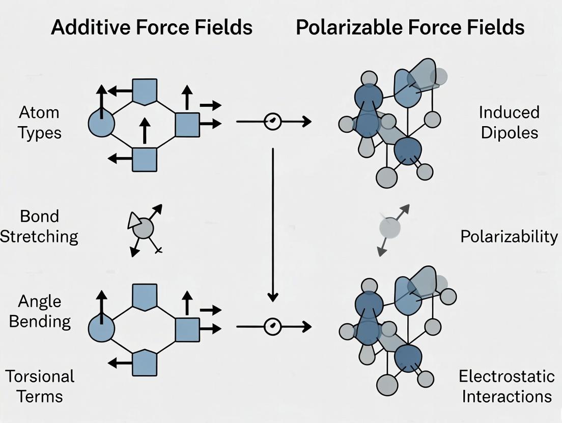
Understanding the Core Physics: Fixed Charges vs. Responsive Electron Clouds

This whitepaper details the foundational principles of classical additive (non-polarizable) force fields, which have underpinned molecular modeling for decades. This exploration exists within a critical research thesis comparing additive force fields with the emerging paradigm of polarizable force fields. While additive models, with their computational efficiency, have driven progress in structural biology and drug discovery, their core simplification—the use of fixed point charges and pairwise summation—is a significant limitation. The broader thesis argues that for systems where electronic polarization is critical (e.g., membrane interfaces, ion binding, spectroscopy), polarizable force fields, though computationally demanding, offer a necessary path toward quantitative accuracy.

Core Tenets: Point Charges and Pairwise Summation

The Concept of Fixed Point Charges

In additive force fields, the complex electron distribution of an atom or group is represented by a single, fixed, partial charge (e.g., +0.42 e). This charge is assigned a priori, typically derived from quantum mechanical calculations and/or empirical fitting to reproduce experimental observables like dipole moments or crystal lattice energies. Once assigned, it remains constant regardless of the atom's changing chemical environment during a simulation.

The Principle of Pairwise Summation (Superposition)

The total non-bonded potential energy (electrostatic + van der Waals) of an N-particle system is calculated as the sum of energies between all unique pairs of atoms (i,j). [ E{\text{total}} = \sum{i=1}^{N-1} \sum{j>i}^{N} \left[ \frac{qi qj}{4\pi\epsilon0 r{ij}} + 4\epsilon{ij} \left( \left(\frac{\sigma{ij}}{r{ij}}\right)^{12} - \left(\frac{\sigma{ij}}{r{ij}}\right)^6 \right) \right] ] The first term is the Coulombic electrostatic energy. The second is the Lennard-Jones potential for van der Waals interactions. Crucially, many-body effects are absent; the interaction between atoms i and j is entirely independent of the position or identity of a third atom k.

Quantitative Comparison of Common Additive Force Fields

Table 1: Characteristics of Major Additive Biomolecular Force Fields

Force Field	Primary Domain	Charge Derivation Method	Key Functional Form & Features	Typical Application
AMBER (ff19SB)	Proteins, DNA/RNA	HF/6-31G* (RESP)	Modified Lennard-Jones; Extensive dihedral parameterization.	Protein folding, protein-ligand binding.
CHARMM (C36/C36m)	Biomolecules, Lipids	MP2/cc-pVTZ (model compounds)	Lennard-Jones 6-12; Coupled with TIP3P/TIP4P water.	Membrane simulations, integral membrane proteins.
OPLS (OPLS4)	Drug-like molecules, Proteins	IPolQ (scaling charges in solution)	Lennard-Jones 6-12; Optimized for liquid-state properties.	Free energy perturbation (FEP) for drug discovery.
GAFF	Small organic molecules	AM1-BCC (semi-empirical)	AMBER-style; General purpose for ligands.	Parameterization of drug candidates for docking/MD.

Table 2: Performance Metrics of Additive Force Fields on Standard Test Sets (Representative Data)

Benchmark Test	AMBER ff19SB	CHARMM36m	OPLS4	Experimental Reference	Limitation Highlighted
Protein Backbone RMSD (Å) (on 20 test proteins)	1.07 ± 0.14	1.12 ± 0.19	1.05 ± 0.16	Crystal/NMR structures	Limited conformational sampling fidelity.
ΔG of Hydration (kcal/mol) (MUE for small molecules)	1.1	0.9	0.7	Solvation free energies	Accuracy depends on charge model & vdW terms.
Ion Binding Site Geometry (e.g., Zn²⁺)	Often requires non-bonded fixes	Often requires non-bonded fixes	Often requires non-bonded fixes	High-resolution X-ray	Fixed charges fail to model ion-induced polarization.
Dielectric Response	~3-5 (low, uniform)	~3-5 (low, uniform)	~3-5 (low, uniform)	~78 (water, high)	Inability to reproduce bulk solvent polarization.

Experimental Protocols for Validating Additive Force Fields

Protocol 1: Parameterization and Validation of Partial Atomic Charges

• Quantum Mechanics (QM) Target Data Generation: Perform ab initio (e.g., MP2/cc-pVTZ) or DFT calculations on the target molecule or representative fragment in vacuum. Key calculation: Electrostatic Potential (ESP) on a grid surrounding the molecule.
• Charge Fitting: Use an algorithm like Restrained Electrostatic Potential (RESP) to fit atomic point charges to reproduce the QM-derived ESP, typically with constraints (e.g., equivalent hydrogens get identical charges) and penalties for large charges to improve transferability.
• Validation: Calculate the molecular dipole moment from the fitted charges and compare to the QM dipole moment. For solvated systems, compute the hydration free energy (ΔG_hyd) via alchemical free energy simulation (e.g., Thermodynamic Integration) and compare to experimental database values.

Protocol 2: Benchmarking Protein Force Field Accuracy

• Test Set Curation: Assemble a diverse set of high-resolution protein crystal structures (e.g., 20-50 proteins). Prepare structures with consistent protonation states and missing loop modeling.
• Molecular Dynamics Simulation: Solvate each protein in a TIP3P water box, add ions to neutralize. Energy minimize, equilibrate (NVT then NPT ensembles at 300K, 1 bar), and run a production simulation of 1 μs per system using a GPU-accelerated MD engine (e.g., OpenMM, AMBER, GROMACS).
• Analysis:
  • Backbone RMSD & RMSF: Calculate the root-mean-square deviation/fluctuation of protein backbone atoms relative to the starting crystal structure.
  • NMR Observables: Compute backbone J-couplings (³J_HN-HA) and residual dipolar couplings (RDCs) from the simulation trajectory and compare to experimental NMR data, if available.
  • χ¹ Rotamer Populations: Compare the sidechain dihedral angle distributions to those in high-resolution structural databases.

Protocol 3: Binding Free Energy (ΔG_bind) Calculation for Drug Discovery

• System Setup: Prepare simulation boxes for the protein-ligand complex, the free ligand in solution, and the free protein in solution (often omitted via double-decoupling methods).
• Alchemical Transformation: Use Free Energy Perturbation (FEP) or Thermodynamic Integration (TI). A coupling parameter (λ) is used to gradually "turn off" the ligand's interactions in the complex state and "turn on" its interactions in the solvated state.
• Simulation: Run a series of parallel simulations at different λ windows. Use Hamiltonian replica exchange (FEP/HRE) to improve sampling.
• Analysis: Use the Bennett Acceptance Ratio (BAR) or Multistate BAR (MBAR) method to compute the free energy difference between the coupled and decoupled states, yielding ΔGbind. Validate against a known series of ligands with experimentally measured IC₅₀ or Kd values.

Diagram: Additive vs. Polarizable Force Field Logic

Title: Logic Flow of Additive vs Polarizable Force Field Selection

Diagram: Free Energy Perturbation (FEP) Workflow

Title: Free Energy Perturbation (FEP) Protocol for Binding Affinity

The Scientist's Toolkit: Research Reagent Solutions

Table 3: Essential Materials and Software for Force Field Research & Application

Item/Category	Specific Examples	Function/Benefit
Force Field Parameter Sets	AMBER ff19SB, CHARMM36, OPLS4, GAFF2	Provides the foundational equations and atom-type-specific parameters (mass, charge, bonds, angles, dihedrals, non-bonded) for MD simulations.
Quantum Chemistry Software	Gaussian, GAMESS, ORCA, Psi4	Used to generate ab initio target data (ESP, conformational energies) for force field parameterization and charge derivation.
Molecular Dynamics Engines	AMBER, GROMACS, NAMD, OpenMM, CHARMM	Software that performs the numerical integration of Newton's equations of motion using the force field. OpenMM enables GPU acceleration.
Force Field Parameterization Tools	Antechamber (for GAFF), ffTK (CHARMM), ParamChem (CGenFF)	Automates the process of assigning atom types, generating parameters, and deriving charges for novel molecules.
Alchemical Free Energy Packages	pmemd (AMBER), somd (OpenMM), FEP+ (Schrödinger), CHARMM/FEP	Specialized modules or workflows designed to run and analyze FEP or TI calculations for solvation/binding free energies.
Validation Databases	PDB (structures), SPICE (QM datasets), FreeSolv (ΔG_hyd), PLANTS (protein-ligand affinities)	Curated experimental or QM reference data used to benchmark and validate force field performance.
Specialized Fixes for Ions/Metals	12-6-4 Li/Mg/Zn parameters (AMBER), CMAP (CHARMM), Non-bonded Fix (NBfix)	Corrections applied to standard additive force fields to improve behavior of divalent ions or protein backbone dihedrals without full polarization.

This whitepaper provides an in-depth technical examination of molecular polarizability—the propensity of a molecule's electron cloud to distort under an external electric field. Framed within the ongoing research debate concerning additive versus polarizable force fields, this document details the theoretical foundations, computational models, and experimental validations of electronic response. It underscores the critical importance of incorporating polarizability for accurate molecular simulations in drug discovery and materials science, where environmental changes are pivotal.

Classical molecular mechanics force fields are the workhorses of computational chemistry and structural biology. Traditionally, additive force fields (e.g., CHARMM36, AMBER ff14SB) treat electrostatic interactions using fixed, pre-assigned atomic partial charges. This model assumes that a charge distribution is invariant, regardless of the molecule's conformation or environment (solvent, protein pocket, membrane). While computationally efficient, this approximation fails to capture electronic polarization—the redistribution of electron density in response to local electric fields from surrounding atoms, ions, or solvents.

Polarizable force fields explicitly model this response, allowing charge distributions to adapt dynamically. This paradigm shift aims to address known deficiencies of additive models in simulating:

• Binding free energies of ligands to proteins.
• Properties of ionic liquids and interfaces.
• Dielectric constants of bulk solvents.
• Phase transitions and spectroscopy.

The core physical property underlying these models is the polarizability tensor (α).

Theoretical Foundations of Polarizability

Definition and Governing Physics

The electronic polarizability (α) quantifies the linear relationship between an induced dipole moment (μind) and an applied static electric field (E): μind = αE In the SI system, α has units of C·m²·V⁻¹ (often reported in the atomic unit of bohr³, where 1 bohr³ ≈ 1.6488 × 10⁻⁴¹ C·m²·V⁻¹). For fields of high intensity, the non-linear hyperpolarizability terms become significant.

The energy (U) associated with polarization in a field is: U = -½ α E²

Key Quantum Mechanical Descriptions

Polarizability is an intrinsic quantum mechanical property. For a molecule in state n, the tensor components can be expressed via sum-over-states perturbation theory: [ \alpha{\rho\sigma}(0;0) = \frac{2}{\hbar} \sum{m \neq n} \frac{\langle n | \hat{\mu}\rho | m \rangle \langle m | \hat{\mu}\sigma | n \rangle}{\omega{mn}} ] where (\omega{mn}) is the transition frequency between states n and m, and (\hat{\mu}) is the dipole moment operator.

In practice, polarizability is computed using finite-field methods (applying a numerical field to a quantum chemistry calculation) or, more commonly, linear response theories (e.g., coupled-perturbed Hartree-Fock/Kohn-Sham) within software packages like Gaussian, PSI4, or DALTON.

Quantitative Data: Polarizabilities of Common Molecular Groups

Table 1: Mean Isotropic Polarizabilities (〈α〉/ a.u.) for Key Chemical Fragments. Data compiled from recent benchmark studies using DFT (ωB97X-V/ aug-cc-pVTZ).

Molecular Fragment/Atom	〈α〉 (a.u.)	Notes
Alkane (-CH₂-)	10.2 ± 0.3	Incremental value in a chain
Aromatic C (in benzene)	12.1 ± 0.5	Highly conjugated systems show larger response
Water (H₂O)	9.8	Strongly anisotropic; value is orientationally averaged
Na⁺ ion	1.0	Closed-shell ions have very low polarizability
Cl⁻ ion	~35.0	Large, diffuse anions are highly polarizable
Peptide backbone (NH–CO)	15.5 ± 1.0	Depends on secondary structure

Computational Models for Polarizability in Force Fields

Three principal methodologies are employed to incorporate polarizability in molecular simulations.

1. Induced Point Dipoles: Atomic polarizabilities are assigned, and interacting induced dipoles are calculated self-consistently.

• Protocol (Typical SCF Iteration):
  • Initialize induced dipoles μind⁽⁰⁾ = 0.
  • Calculate total electric field Eᵢ at each polarizable site i from static charges and other induced dipoles.
  • Update induced dipoles: μind,ᵢ⁽ⁿ⁺¹⁾ = αᵢ (Eᵢ⁽ⁿ⁾).
  • Check for convergence: |μind⁽ⁿ⁺¹⁾ - μind⁽ⁿ⁾| < tolerance (e.g., 1.0e-4 D).
  • Repeat steps 2-4 until convergence. Use extrapolation (e.g., Jacobi/GS) or direct inversion to accelerate.
• Example Force Fields: AMOEBA, CHARMM Drude.

2. Drude Oscillator (Charge-on-Spring): A massless, charged "Drude" particle is attached to its parent atom via a harmonic spring, representing a displaceable electron cloud.

• Protocol (Extended Lagrangian Dynamics):
  • For each polarizable atom, introduce a Drude particle with charge -qD and parent atom charge +qD.
  • Assign a harmonic spring constant k_D between them (typically 1000-5000 kcal/mol/Ų).
  • The Drude particle's position is propagated as a dynamical variable (with a "cold" thermostat) or minimized instantaneously at each MD step.
  • The induced dipole is μind = qD * d, where d is the displacement vector.
• Example Force Fields: CHARMM Drude, Classical Drude Oscillator (POL3).

3. Fluctuating Charges (Electronegativity Equalization): Atomic charges fluctuate in response to the instantaneous chemical potential of the environment to equalize electronegativity.

• Protocol (Chemical Potential Equilibration):
  • Define atomic hardness parameters (ηᵢ) and electronegativities (χᵢ).
  • For a given molecular geometry, the total energy is expressed as a function of atomic charges {qᵢ}.
  • Minimize energy subject to total charge constraint using Lagrange multipliers.
  • Solve the resulting linear equations for {qᵢ} at each simulation step.
• Example Model: ReaxFF, QTPIE.

Table 2: Comparison of Polarizable Force Field Methodologies.

Model	Computational Cost	Key Advantages	Key Challenges
Induced Dipole	High (requires SCF)	Physically intuitive, accurate for anisotropic systems	Polarizability catastrophe at short range, high cost
Drude Oscillator	Moderate (~2x additive)	Simple physics, easy integration into MD	Requires dual thermostats, parameterization of springs
Fluctuating Charges	Low-Moderate	Captures charge transfer effects	Less direct link to polarizability, parameterization complexity

Experimental Protocols for Validating Polarizability

Computational models require experimental validation. Key methods include:

4.1 Dielectric Constant Measurement:

• Objective: Measure the static dielectric constant (ε₀) of a pure liquid or solution, which is directly related to the molecular dipole moment and polarizability via the Clausius-Mossotti equation.
• Protocol (Capacitance Method):
  • Fill a precision parallel-plate capacitor cell with the sample liquid.
  • Measure the capacitance (C) of the cell using a high-precision LCR meter at multiple frequencies (typically 1 kHz - 1 MHz).
  • Measure the capacitance of the empty cell (Cvac).
  • Calculate the relative permittivity (dielectric constant): εr = C / Cvac.
  • Relate εr to the molecular polarizability volume via: (εr - 1)/(εr + 2) = (4π/3) N_A ρ α' / M, where ρ is density, M is molar mass, and α' is the orientationally averaged polarizability.

4.2 Refractive Index Measurement:

• Objective: Determine the frequency-dependent electronic polarizability (at optical frequencies) via the refractive index (n).
• Protocol (Abbe Refractometer):
  • Calibrate the refractometer using a standard (e.g., distilled water, nD²⁰ = 1.3330).
  • Place a few drops of the liquid sample on the main prism and close the daylighting plate.
  • Adjust the eyepiece until the crosshairs are sharp. Align the boundary between light and dark fields to the intersection of the crosshairs.
  • Read the refractive index value directly from the scale to four decimal places at a controlled temperature (usually 20°C or 25°C).
  • Apply the Lorentz-Lorenz relation: (n² - 1)/(n² + 2) = (4π/3) NA ρ α / M.

4.3 X-ray or Neutron Diffraction with Multipole Refinement:

• Objective: Obtain experimental electron density maps to derive static dipole moments and validate induced charge distributions in crystals.
• Protocol (High-Resolution X-ray Diffraction):
  • Grow a high-quality single crystal (~0.1-0.3 mm) of the target molecule.
  • Collect diffraction data on a modern diffractometer (e.g., Mo Kα, λ = 0.71073 Å) at low temperature (e.g., 100 K) to high resolution (sin θ/λ > 1.0 Å⁻¹).
  • Refine the structure using the Hansen-Coppens multipole model. This model partitions electron density into spherical core, valence, and deformation densities.
  • Analyze the refined multipole parameters (dipole, quadrupole moments) to compute the molecular electrostatic potential and static polarization in the crystal environment.

Visualizing Concepts and Workflows

Polarizable vs. Additive FF Paradigm (77 chars)

Induced Dipole SCF Cycle (46 chars)

The Scientist's Toolkit: Research Reagent Solutions

Table 3: Essential Materials and Tools for Polarizability Research.

Item	Function/Brand Example	Brief Explanation of Role
High-Precision LCR Meter	Keysight E4980AL	Measures capacitance and impedance for dielectric constant determination.
Abbe Refractometer	ATAGO NAR-1T Liquid	Precisely measures refractive index of liquids to 4 decimal places.
Quantum Chemistry Software	Gaussian 16, PSI4, ORCA	Computes reference ab initio polarizability tensors and dipole moments for parameterization.
Polarizable MD Software	OpenMM, NAMD (w/ AMOEBA/Drude), TINKER	Molecular dynamics engines that support polarizable force field Hamiltonians.
High-Resolution XRD System	Rigaku Synergy-S, Bruker D8 VENTURE	Collects single-crystal X-ray diffraction data for experimental electron density analysis.
Parametrization Platform	Force Field Toolkit (fFTK) in VMD, PyRED (for Drude)	Aids in systematic derivation of polarizable force field parameters from QM data.
Reference Polarizability Database	NIST Computational Chemistry Comparison (CCCBDB)	Repository for experimental and high-level computational polarizability benchmarks.

Incorporating polarizability is a essential step towards achieving chemical accuracy in molecular simulations. While additive force fields remain valuable for high-throughput screening and large-scale system equilibration, polarizable models are becoming increasingly tractable and necessary for quantitative predictions in drug design—particularly for binding affinity calculations, ion channel studies, and spectroscopy. The future lies in the continued development of efficient, scalable, and robustly parameterized polarizable force fields, potentially augmented with machine learning techniques to capture even more complex electronic responses. This will bridge the gap between the computational efficiency of classical mechanics and the accuracy of quantum mechanics.

This whitepaper details the pivotal evolution from classical additive force fields, exemplified by CHARMM and AMBER, to advanced polarizable models such as AMOEBA and CHARMM-DRK. Framed within the broader thesis of additive versus polarizable force field research, this document provides a technical guide for researchers and drug development professionals. Polarizable force fields address the critical limitation of additive models—the fixed-point charge approximation—by explicitly modeling electronic polarization, leading to superior accuracy in simulating electrostatic interactions, ligand binding, and heterogeneous environments like protein-solvent interfaces.

Classical molecular mechanics force fields partition energy into bonded and non-bonded terms. The dominant additive models, CHARMM and AMBER, utilize a fixed, atom-centered partial charge distribution. This approximation treats electrostatic interactions as pairwise additive, neglecting the intrinsic response of electron density to a changing environment.

Core Limitation: The inability to model electronic polarization leads to systematic errors in:

• Binding affinity calculations (over/under-estimation)
• Properties of ions in solution
• Interfacial systems (membrane-protein, solvent-protein)
• Spectroscopy (IR, NMR) prediction accuracy

This necessitated the development of polarizable force fields, which explicitly account for the redistribution of charge in response to the local electric field.

Theoretical Foundations of Polarizability

Polarization Methods

Three primary methods are employed to incorporate polarizability:

Method	Core Principle	Mathematical Formulation (Simplified)	Key Advantage	Key Disadvantage
Induced Point Dipoles	Atoms possess isotropic polarizabilities; external field induces dipole moment (µ_ind).	µind = α · Elocal	Physically intuitive, well-established.	Can suffer from "polarization catastrophe" (over-polarization) at short range.
Fluctuating Charges (Charge Equilibration)	Atomic charges fluctuate to equalize electronegativity across the molecule.	Δχi + ∑j Jij Δqj = 0	Charge transfer is natural, computationally efficient.	Less accurate for directional polarization (e.g., π-systems).
Classical Drude Oscillators	A massless, charged "Drude" particle is attached to a core atom via a harmonic spring.	Fspring = -k (rcore - r_Drude)	Effectively models anisotropic polarization, avoids catastrophe.	Introduces extra degrees of freedom; requires extended Lagrangian methods.

The Thole Damping Function

A critical component for induced dipole models is the Thole damping function. It prevents the "polarization catastrophe" by scaling the dipole field tensor at short distances, ensuring model stability.

Evolution to Specific Polarizable Models

The AMOEBA (Atomic Multipole Optimized Energetics for Biomolecular Applications) Model

AMOEBA employs a permanent atomic multipole expansion (up to quadrupole) and induced atomic dipoles with Thole damping.

Key Features:

• Permanent Electrostatics: Uses distributed multipoles (charge, dipole, quadrupole) from ab initio calculations for superior representation of molecular electrostatic potentials (MEP).
• Polarization: Induced point dipoles with Thole damping.
• vdW: A buffered 14-7 potential form.

Parameterization Workflow:

• Target data from high-level quantum mechanical (QM) calculations (e.g., MP2/aug-cc-pVTZ).
• Electrostatic parameters fitted to reproduce QM-derived MEP and molecular dipole moments in various conformations.
• van der Waals and torsion parameters optimized to match QM conformational energies and experimental condensed-phase properties (density, heat of vaporization).

The CHARMM-Drude (or CHARMM-DRK) Model

The CHARMM-Drude model uses the classical Drude oscillator formalism, where an atom's polarizability is represented by a charged Drude particle connected to its core.

Key Features:

• Polarizability: Each polarizable atom has a Drude particle (charge -qD) attached to its core (charge +qD). The induced dipole is µind = qD * (rDrude - rcore).
• Anisotropy: Achieved by assigning anisotropic spring constants or using multiple Drude particles.
• Thermostat: Requires a dual-Langevin thermostat (or extended Lagrangian) to maintain low temperature for Drude particles, separating their degrees of freedom from atomic motion.

Quantitative Performance Comparison

Table 1: Theoretical & Performance Comparison of Force Field Families

Property	Additive (CHARMM36/AMBER ff19SB)	AMOEBA (2013, 2018)	CHARMM-Drude (2019, 2022)
Electrostatic Formulation	Fixed point charges (monopoles)	Permanent atomic multipoles + induced dipoles	Fixed + mobile Drude charges (effective induced dipoles)
Polarization Formalism	Mean-field (implicit via high dielectric constant)	Explicit, via induced point dipoles (Thole damped)	Explicit, via classical Drude oscillators
Typical Relative Speed	1.0x (Baseline)	5-10x slower	3-6x slower
Ion Binding Free Energy (kcal/mol error)	High (2-5)	Low (< 1-2)	Low (< 1-2)
Liquid Phase Dielectric Constant	Often over/under-estimated	Accurate (±~5%)	Accurate (±~5%)
NMR J-Coupling Prediction	Poor correlation with experiment	Good to excellent correlation (R² > 0.9)	Good correlation (R² > 0.85)

Table 2: Representative Benchmarking Results (Condensed)

System/Property	Experimental Value	Additive FF Result	AMOEBA Result	CHARMM-Drude Result	Citation (Example)
Water Dielectric Constant (ε)	78.4	~90-100 (TIP3P)	78 ± 3	80 ± 2	Ponder, 2010; Lemkul, 2016
Na⁺ Hydration Free Energy (kcal/mol)	-98	-120 to -80	-100 ± 3	-97 ± 2	Grossfield, 2003; Savelyev, 2014
Protein Backbone J-couplings (Hz RMSD)	-	1.5 - 2.5	0.4 - 0.8	0.6 - 1.0	Showalter, 2007; Huang, 2014

Experimental Protocols for Validation

Protocol: Calculation of Ion Hydration Free Energies (Thermodynamic Integration)

Purpose: Validate electrostatic and polarization response in aqueous solution.

• System Setup: Place a single ion in a cubic box of water (e.g., 1000 molecules). Use periodic boundary conditions.
• Alchemical Pathway: Define a coupling parameter λ (0→1) that scales the ion's non-bonded interactions with its environment from "fully interacting" to "fully decoupled."
• Simulation: Perform a series of molecular dynamics (MD) simulations at discrete λ windows (e.g., λ = 0.0, 0.1, 0.2, ... 1.0). At each window, equilibrate for 2 ns, then produce 10 ns of production data.
• Free Energy Analysis: Use the Bennett Acceptance Ratio (BAR) or Multistate BAR (MBAR) method to compute the ensemble average of ∂H/∂λ and integrate over λ to obtain the total free energy change (ΔG_hydration).
• Comparison: Compare computed ΔG_hydration to high-accuracy experimental references.

Protocol: NMR J-Coupling Calculation from MD Trajectories

Purpose: Assess the accuracy of torsional sampling and electronic environment.

• Trajectory Generation: Run a long-timescale (≥ 1 µs) MD simulation of the target molecule (e.g., a protein or peptide) in explicit solvent.
• Frame Selection: Extract thousands of uncorrelated snapshots from the equilibrated trajectory.
• QM Calculation on Snapshots: For each snapshot, perform a geometry optimization (constrained on heavy atoms) followed by a single-point energy and NMR calculation (e.g., using DFT methods like B3LYP/6-31G) on the molecule of interest (often in vacuum or with a continuum solvent model).
• Averaging: Compute the Boltzmann-weighted average of the QM-derived J-couplings across all snapshots.
• Validation: Plot computed vs. experimental J-couplings and calculate the correlation coefficient (R²) and root-mean-square deviation (RMSD).

Visualizations

Title: Evolution from Additive to Polarizable Force Fields

Title: Polarizable Force Field Parameterization Workflow

The Scientist's Toolkit: Research Reagent Solutions

Table 3: Essential Software & Resources for Polarizable FF Research

Item Name	Category	Primary Function	Notes / Key Provider
OpenMM	MD Engine	Highly optimized, GPU-accelerated simulation. Supports AMOEBA and Drude models.	Primary platform for AMOEBA development & benchmarks.
CHARMM/OpenCHARMM	MD Engine	Native support for CHARMM-Drude model. Comprehensive tool for setup, simulation, and analysis.	Official suite for CHARMM force fields.
TINKER/TINKER-HP	MD Engine	Specialized software for the AMOEBA force field. TINKER-HP enables high-performance parallel scaling.	Ponder group; key for AMOEBA applications.
Gaussian, ORCA, Psi4	QM Software	Generate target data for parameterization (MEP, conformational energies, polarizabilities).	Essential for force field development.
ForceField Toolkit (fFTK)	Parameterization	Plugin for CHARMM GUI and OpenMM to assist in developing new force field parameters.	Automates parts of the parameterization workflow.
CHARMM-GUI Drude Prepper	System Setup	Web-based tool to build and equilibrate complex systems (proteins, membranes) with the Drude model.	Drastically simplifies setup for end-users.
MBAR, pymbar	Analysis Tool	Perform free energy perturbation (FEP) and thermodynamic integration (TI) analysis.	Critical for computing binding affinities and validation.
VMD/ChimeraX	Visualization	Visualize trajectories, analyze structures, and prepare figures.	Standard for molecular graphics.

The development of molecular force fields represents a foundational pursuit in computational chemistry and biophysics. The central thesis in modern force field research hinges on the dichotomy between traditional additive models and advanced polarizable frameworks. Additive force fields, which assign static, fixed partial charges to atoms, have driven decades of progress in molecular dynamics (MD) simulations. However, their inherent limitation—the inability to respond to changes in the local electrostatic environment—becomes critically apparent in heterogeneous systems such as protein-ligand binding pockets, lipid bilayer interfaces, and electrochemical environments. This whitepaper articulates the physical imperative for explicit polarizability, detailing why fixed charges are fundamentally insufficient for modeling complex, heterogeneous environments with quantitative accuracy, and provides a technical guide to the associated evidence and methodologies.

The Fundamental Limitation of Fixed Charges

In additive force fields (e.g., CHARMM36, AMBER ff14SB, OPLS-AA), the electrostatic potential is represented by a sum of Coulombic interactions between fixed point charges centered on atomic nuclei. This model assumes that the electron density of an atom or molecule is rigid and does not redistribute in response to its surroundings—an approximation valid only in homogeneous, isotropic environments of similar dielectric constant.

The failure of this model in heterogeneous environments is physical and predictable:

• Dielectric Discontinuity: At interfaces (e.g., water-membrane, protein-solvent), the dielectric constant changes abruptly. A fixed-charge model cannot capture the induced polarization (electronic and atomic) that fundamentally modulates electrostatic interactions.
• Many-body Effects: Additive force fields are effectively pairwise additive. They ignore many-body polarization, where the charge distribution on a molecule is influenced by the collective field of all surrounding particles, not just pairwise interactions.
• Charge Transfer: In tightly bound complexes (e.g., metal ions in active sites, strong hydrogen bonds), partial electron sharing occurs, which is a quantum mechanical effect impossible to model with static charges.

Recent search results from the literature consistently highlight that fixed-charge errors are most pronounced in simulating ion permeation through channels, binding affinities of charged ligands, and the structure of interfacial water.

Quantitative Evidence: Polarizable vs. Additive Force Fields

The following tables summarize key quantitative findings from recent experimental validations and simulation benchmarks.

Table 1: Performance in Biomolecular Binding Free Energy Calculations

System (Ligand-Protein)	Additive FF Error (kcal/mol)	Polarizable FF Error (kcal/mol)	Experimental Reference Method	Key Finding
Benzamidine-Trypsin	2.5 - 4.0	0.5 - 1.2	ITC / Thermofluor	Polarizable models capture charge penetration and exchange effects.
Oxoanion (SO₄²⁻) Binding Protein	> 3.0 (incorrect ranking)	< 1.0 (correct ranking)	Crystallography & Affinity	Fixed charges overestimate anion binding due to lack of polarization damping.
Drug Fragment (charged) in GPCR Pocket	Poor correlation (R² < 0.3)	Strong correlation (R² > 0.8)	SPR Competition Assay	Polarizability critical for heterogeneous, low-dielectric binding sites.

Table 2: Physical Property Benchmarks in Heterogeneous Environments

Property & System	Additive FF Result	Polarizable FF Result	Experimental Value	Implication
Ion Permeation Free Energy (K⁺ channel)	Barrier too high by ~8 kcal/mol	Barrier within 2 kcal/mol	Electrophysiology Reversal Potential	Fixed charges exaggerate ion desolvation penalty.
Interfacial Water Dipole Moment (Air-Water)	Constant (~2.3 D)	Reduced at interface (~2.0 D)	SFG Spectroscopy & Theory	Polarization response to asymmetric field is captured.
Peptide Backbone ¹⁵N NMR Shift (in membrane)	Poor agreement (RMSD > 8 ppm)	Good agreement (RMSD < 3 ppm)	Solid-State NMR	Polarizable models accurately report on local electrostatic fields.

Core Methodologies for Polarizable Force Field Development & Validation

Protocol: Induced Dipole-Based Polarizable MD Simulation (e.g., AMOEBA, Drude)

Objective: To simulate a solvated protein-ligand system with explicit electronic polarization.

• System Preparation:

  • Obtain protein and ligand structures from PDB/ligand database.
  • Parameterize the ligand using the polarizable force field's protocol (e.g., for AMOEBA: derive distributed multipoles from quantum mechanical (QM) electrostatic potential; for Drude: assign atomic polarizabilities and link to Drude oscillators).
  • Solvate the complex in a pre-equilibrated box of polarizable water (e.g., SWM4-NDP, TIP4P-FQ).

• Simulation Setup:

  • Employ a dual-thermostat setup for Drude oscillators (Nose-Hoover for real atoms, Langevin for Drudes) to maintain a low "temperature" for the Drude particles (~1 K), representing electronic degrees of freedom.
  • For induced dipole models (AMOEBA), use a variational solver to converge dipoles self-consistently at each step.
  • Use a particle-mesh Ewald (PME) method extended for polarizable interactions (e.g., Thole-damped interactions).

• Production Run & Analysis:

  • Run MD for >100 ns. Monitor convergence of binding interface properties.
  • Key analysis: Calculate time-dependent dipole moments of residues/ligands, compare electrostatic potential maps to QM data, and compute binding free energies via FEP/MBAR.

Protocol: Benchmarking via Liquid Property Calculations

Objective: To validate the fundamental physics of a polarizable water model.

• Simulation Ensemble:

  • Simulate a box of 256-1000 water molecules using NPT ensemble (298 K, 1 bar) for 10-20 ns.

• Property Calculation:

  • Dielectric Constant: Calculate the fluctuation of the total system dipole moment.
  • Diffusion Coefficient: From mean squared displacement of oxygen atoms.
  • Air-Water Interfacial Tension: Simulate a water slab in vacuum, calculate pressure tensor components.

• Validation:

  • Compare calculated properties (dielectric constant, diffusion coefficient, density, vaporization enthalpy, interfacial tension) against high-fidelity experimental data. A polarizable model must simultaneously reproduce bulk and interfacial properties.

Visualizing the Polarization Response

Diagram Title: Model Performance in Different Environments

Diagram Title: Polarizable Force Field Development Workflow

The Scientist's Toolkit: Essential Research Reagents & Solutions

Table 3: Key Reagents & Computational Tools for Polarizable Simulations

Item / Solution	Function / Purpose	Example (Vendor/Software)
Polarizable Force Field Parameters	Provides atomic polarizabilities, Thole damping factors, and (optionally) multipole moments for biomolecules and small molecules.	AMOEBA (OpenMM, Tinker), CHARMM Drude (CHARMM-GUI), GROMOS Polarizable 2017H66.
Polarizable Water Model	Explicitly models water with polarizable sites to correctly represent solvent response.	SWM4-NDP (Drude), TIP4P-FQ (Fluctuating Charge), AMOEBA water.
QM Software	To compute target data (electrostatic potential, polarizability tensors) for parameterization.	Gaussian, GAMESS, PSI4, ORCA.
MD Engine with Polarization Support	Simulation software that can integrate the equations of motion for polarizable models.	OpenMM (AMOEBA), NAMD (Drude), Tinker-HP (AMOEBA), CHARMM (Drude).
System Building & Parameterization Tool	Automates the complex process of assigning polarizable parameters to novel molecules or biomolecular systems.	CHARMM-GUI Drude Prepper, Poltype (for AMOEBA), LigParGen (OPLS with CM1A charges).
Enhanced Sampling Suite	To overcome sampling challenges in binding free energy calculations with more expensive polarizable models.	PLUMED (for metadynamics, FEP), NAMD's FEP module (for Drude).
High-Performance Computing (HPC) Resources	Essential due to the 3-10x computational cost of polarizable simulations versus additive ones.	GPU clusters (NVIDIA A100/V100), National supercomputing centers (XSEDE, PRACE).

Within the ongoing research thesis on additive (fixed-charge) versus polarizable force fields (FFs), the incorporation of electronic polarization is critical for accurate simulations of biomolecular interactions, spectroscopy, and heterogeneous environments. Additive FFs assign static partial charges, failing to respond to changing electrostatic environments. Polarizable FFs address this by allowing charge distributions to adapt, significantly improving the description of phenomena like dielectric constants, ion binding, and solvent interactions. This guide details the three main paradigms for implementing polarizability: Drude Oscillators, Induced Point Dipoles, and Fluctuating Charges.

Core Principles and Mathematical Formalisms

Drude Oscillators (Classical Drude Model)

In this model, polarization is represented by attaching a massless, charged "Drude particle" (typically a negative charge) to each polarizable atom via a harmonic spring. The Drude particle can displace in response to the local electric field, inducing a dipole moment. The core atom carries a charge of ( qc ) and the Drude particle a charge of ( qD = -qD ), with ( qc + qD = q{total} ) (the static atomic charge). The induced dipole ( \mu{ind} = qD * rD ), where ( rD ) is the displacement vector. The potential energy includes a harmonic spring term: ( U{spring} = \frac{1}{2} kD |rD|^2 ). The polarizability ( \alpha ) is related to the force constant by ( \alpha = qD^2 / k_D ).

Induced Point Dipoles

This model assigns an inducible point dipole to specific atomic sites. The dipole moment ( \mui ) at atom ( i ) is proportional to the total electric field ( Ei ) at that site: ( \mui = \alphai Ei^{total} ). The total field is the sum of the external field and the field from all other permanent and induced dipoles in the system: ( Ei^{total} = Ei^{static} - \sum{j \neq i} T{ij} \muj ), where ( T_{ij} ) is the dipole field tensor. This leads to a set of coupled equations that must be solved self-consistently (usually iteratively) or via extended Lagrangian methods.

Fluctuating Charges (FQ or Charge Equilibration)

Also known as chemical potential equilibration or electronegativity equalization, this model treats atomic partial charges as dynamic variables that fluctuate to equalize the instantaneous chemical potential (electronegativity) across the molecule. The energy is expressed as a Taylor expansion around a reference state: ( E({q}) = \sumi (\chii^0 qi + \frac{1}{2} J{ii}^0 qi^2) + \sum{i{ij}(r{ij}) qi qj ), subject to the constraint of total charge conservation. Minimizing this energy with respect to charges under constraint yields the equilibrated charges at each timestep. Polarization arises from charge transfer between atoms.

Comparative Analysis & Quantitative Data

Table 1: Core Characteristics of Polarizable Models

Feature	Drude Oscillators	Induced Point Dipoles	Fluctuating Charges
Physical Representation	Auxiliary charged particle on a spring.	Point polarizability tensor at atomic center.	Dynamical atomic partial charges.
Primary Mechanism	Displacement of charge.	Induction of dipole moment.	Redistribution of charge (charge flow).
Key Parameter(s)	Drude charge ((qD)), spring constant ((kD)).	Isotropic/anisotropic polarizability ((\alpha_i)).	Electronegativity ((\chii^0)), hardness ((J{ii}^0)).
Energy Term	Harmonic spring: ( \frac{1}{2} kD rD^2 ).	Dipole field interaction: ( -\mui \cdot Ei ).	Charge-dependent: ( \chi q + \frac{1}{2} J q^2 + \sum J{ij}qi q_j ).
Computational Cost	Moderate (extra particles, dual NVE).	High (matrix inversion/iteration for mutual induction).	Moderate (matrix inversion for charge equilibration).
Handles Anisotropy	Via anisotropic spring constants.	Yes, via tensor polarizability.	Implicitly via geometry.
Example FF Implementations	CHARMM Drude FF, AMOEBA (combines with FQ).	AMOEBA (primary), OPLS with IPD.	AMOEBA (secondary), QTPIE, ReaxFF.
Typical Application	Biomolecules (proteins, lipids), solvents.	High accuracy biomolecular & liquid simulations.	Materials, reactive systems, combined models.

Table 2: Performance Benchmark (Representative Data from Literature)

Model & System	System Size	Software (e.g.)	Speed (ns/day) vs Additive	Key Accuracy Improvement
Drude: Lysozyme in Water	~40,000 atoms	NAMD, CHARMM	2-4x slower	Dielectric constant of water, peptide backbone dipole.
Induced Dipole: DHFR	~50,000 atoms	Tinker-HP, OpenMM	5-15x slower	Ion binding free energies, interaction energies.
FQ: Ionic Liquid [BMIM][BF4]	500 ion pairs	CP2K, LAMMPS	3-8x slower	Charge transfer dynamics, vibrational spectra.

Experimental & Computational Protocols

Protocol: Parameterization of a Drude Water Model

• Target Data Selection: Ab initio (e.g., MP2/aug-cc-pVTZ) data for water dimer energies at multiple orientations and distances, monomer polarizability, dipole moment, and bulk properties (density, enthalpy of vaporization, dielectric constant).
• Initial Guess: Assign static charges to O and H atoms. Attach a Drude particle to oxygen. Set initial ( qD ) and ( kD ) based on desired oxygen polarizability (( \alphaO = qD^2/k_D )).
• Force Field Optimization: Use a Monte Carlo or simplex algorithm to iteratively adjust:
  • Static atomic charges.
  • Drude charge ((qD)) and spring constant ((kD)).
  • Lenn-Jones parameters (ε, σ).
• Validation Simulation: Perform molecular dynamics (MD) in an NPT ensemble of ~512 water molecules.
• Property Calculation: Compute bulk density (ρ), enthalpy of vaporization (ΔHvap), static dielectric constant (ε0), and diffusion coefficient (D).
• Iterative Refinement: Compare calculated properties to experimental targets (ρ = 0.997 g/cm³, ΔHvap = 10.52 kcal/mol, ε0 = 78.4) and adjust parameters until agreement is within tolerance.

Protocol: Computing Polarization Energy with an Induced Dipole Model

• System Preparation: Generate coordinates for a target molecule (e.g., a protein-ligand complex) and assign static charges & polarizabilities (from FF, e.g., AMOEBA).
• Calculate Static Field: Compute the electric field ( E_i^{static} ) at each polarizable atom i from all static (permanent) charges in the system.
• Solve Induced Dipoles: For a system of N polarizable sites, solve the ( 3N \times 3N ) linear system: ( \mu = \alpha (E^{static} - T \mu) ), where ( T ) is the dipole field interaction tensor. This is done iteratively: a. Initialize ( \mu = 0 ). b. Compute total field: ( Ei^{total} = Ei^{static} - \sum{j \neq i} T{ij} \muj ). c. Update dipoles: ( \mui^{new} = \alphai Ei^{total} ). d. Repeat steps b-c until ( |\mu^{new} - \mu^{old}| < ) threshold (e.g., 1e-6 D).
• Energy Calculation: Compute the polarization energy: ( U{pol} = -\frac{1}{2} \sumi \mui \cdot Ei^{static} ).
• Analysis: Compare ( U_{pol} ) to the static electrostatic energy to quantify the polarization contribution to binding or solvation.

Visualizations

Diagram Title: Hierarchy and Relationship of Common Force Field Types

Diagram Title: Generalized MD Workflow for Polarizable Force Fields

The Scientist's Toolkit: Research Reagent Solutions

Table 3: Essential Computational Tools for Polarizable MD

Item / Software	Function / Description	Typical Use Case
CHARMM	MD program with robust implementation of the Drude oscillator model.	Simulating lipid bilayers, proteins, and nucleic acids with the CHARMM Drude FF.
Tinker / Tinker-HP	MD package specializing in the AMOEBA polarizable FF (Induced Dipoles + FQ).	High-accuracy studies of biomolecular binding, ion channels, and spectroscopy.
OpenMM	High-performance, GPU-accelerated toolkit supporting AMOEBA and custom forces.	Rapid development and production runs of polarizable simulations on GPUs.
CP2K	Quantum mechanics/molecular mechanics (QM/MM) and MD with FQ support.	Simulating reactive systems, materials, and solid-state interfaces.
LAMMPS	Highly versatile MD code with plugins/user packages for polarizable models.	Large-scale simulations of polymers, nanomaterials, and coarse-grained models.
Force Field Parameter Files (e.g., drude.prm, amoebabio18.xml)	FF-specific parameter files defining polarizabilities, charges, and bonded terms.	Essential input for any polarizable simulation; must match the target system.
Polarization Solvers (e.g., SCF, extended Lagrangian)	Algorithms to compute induced dipoles/charges at each step.	Core computational kernel; choice affects stability, accuracy, and speed.
Visualization Software (VMD, PyMOL)	Tools to analyze trajectories, visualize dipole moments, and charge fluctuations.	Post-simulation analysis to interpret polarization effects on structure/dynamics.

Implementation in Research: Parameterization, Software, and Use Cases

The development of molecular mechanics force fields is fundamentally anchored in the choice between additive (fixed-charge) and polarizable electrostatic models. This choice dictates the entire parameterization workflow. Additive force fields, such as GAFF2 and CHARMM36, assign static partial atomic charges, offering computational efficiency. Polarizable force fields, like AMOEBA and CHARMM Drude, incorporate electronic response through induced dipoles, Drude oscillators, or fluctuating charges, providing superior accuracy for condensed-phase and electrostatic properties at increased computational cost. This guide details the technical workflow for parameterizing both types, emphasizing the iterative fitting to quantum mechanical (QM) data and experimental condensed-phase properties, framed within this critical research dichotomy.

Core Parameterization Workflow

The parameterization of both additive and polarizable force fields follows a hierarchical, multi-target optimization process. The primary divergence lies in the electrostatic parameter set being optimized.

Diagram Title: Force Field Parameterization Decision and Optimization Workflow

Quantum Mechanical Target Data Acquisition

Protocol 2.2.1: Torsional Potential Energy Scan

• System Setup: Select the rotatable bond of interest. Define the dihedral angle.
• QM Calculation: Using software (e.g., Gaussian, ORCA), perform a constrained geometry optimization at fixed dihedral angle intervals (typically 15° or 30°). Hold the target dihedral fixed while relaxing all other coordinates.
• Level of Theory: Employ high-level methods like CCSD(T)/CBS or, more commonly for training sets, DFT with dispersion-corrected functionals (e.g., ωB97X-D/def2-TZVP).
• Output: Relative energy (ΔE) at each angle, constituting the 1-D torsional profile.

Protocol 2.2.2: Intermolecular Interaction Energy (Dimer Scan)

• Dimer Construction: Generate multiple orientations and distances for a pair of molecules (e.g., water-model compound).
• QM Single-Point Energy: Calculate the interaction energy at each geometry: ΔEint = Edimer - (EmonomerA + EmonomerB).
• Basis Set Superposition Error (BSSE): Correct for BSSE using the counterpoise method.
• Level of Theory: Use high-level ab initio methods (MP2, CCSD(T)) with large basis sets, or extrapolate to the complete basis set (CBS) limit.

Protocol 2.2.3: Molecular Electrostatic Potential (ESP) Calculation

• Optimized Geometry: Use a single, optimized molecular geometry (preferably at the MP2/cc-pVTZ or similar level).
• ESP Generation: Compute the QM-derived ESP on a Connolly surface (e.g., at van der Waals radius + probe distance).
• Target for Fitting: This grid of ESP points is the primary target for fitting atomic partial charges (additive) or combined charge/polarizability parameters (polarizable).

Condensed-Phase Property Simulation Protocols

Protocol 2.3.1: Liquid Density (ρ) and Enthalpy of Vaporization (ΔH_vap)

• System Preparation: Build a cubic box containing 500-1000 molecules, using Packmol.
• Equilibration: Run NPT simulation (e.g., 298 K, 1 bar) for 5-10 ns using a barostat (e.g., Berendsen, then Parrinello-Rahman) and thermostat (e.g., Nosé-Hoover).
• Production: Run a further 10-20 ns of NPT simulation, saving coordinates and energies.
• Analysis:
  • ρ: Average the box volume over the production run; calculate mass/volume.
  • ΔHvap: Calculate as ΔHvap = ⟨Egas⟩ - ⟨Eliq⟩ + RT, where ⟨E⟩ is the average potential energy per molecule from gas-phase and liquid-phase simulations, respectively.

Protocol 2.3.2: Dielectric Constant (ε)

• System Preparation: Use the equilibrated liquid box from Protocol 2.3.1.
• Simulation: Run a long NVT simulation (50+ ns) without an applied field.
• Analysis: Calculate the static dielectric constant from the fluctuations of the total dipole moment M of the simulation box: (ε - 1) = (4π/3Vk_BT) (⟨M²⟩ - ⟨M⟩²).

Parameter Optimization Loop

The optimization minimizes a weighted objective function (χ²): χ² = Σi wi (Oi^calc - Oi^target)²

Targets (O_i^target) include QM energies (dimers, torsions) and experimental condensed-phase properties.

Algorithm: Automated tools (e.g., ForceBalance, ParAMS) use gradient-based optimization (e.g., Levenberg-Marquardt) to adjust parameters (charges, Lennard-Jones ε/σ, polarizabilities, torsional force constants) to minimize χ².

Data Presentation: Additive vs. Polarizable Performance

Table 1: Representative Target Data for Small Molecule Parameterization

Target Property	Typical QM/Expt Source	Weight in Optimization	Additive FF Challenge	Polarizable FF Advantage
Torsional Energy Profile	DFT (ωB97X-D/def2-TZVP) Scan	High	May over-stiffen due to mean-field charge	Better captures conformation-dependent electrostatics
Water Dimer & Cluster Energies	CCSD(T)/CBS	High	Can fit dimer well, fails for larger clusters	Consistently accurate across cluster sizes
Molecular Dipole Moment	QM (Gas-Phase)	Medium	Fixed value	Enhanced in condensed phase via induction
Liquid Density (ρ)	Experiment (298 K, 1 atm)	High	Can be fit accurately	Can be fit accurately
Enthalpy of Vaporization (ΔH_vap)	Experiment	High	Often overestimated	More accurate due to many-body polarization
Static Dielectric Constant (ε)	Experiment	Low (Additive), High (Polarizable)	Often under-predicted (e.g., water ~70 vs. expt ~80)	Accurately reproduced (e.g., water ~78)
Diffusion Coefficient (D)	Experiment	Low	Sensitive to van der Waals parametrization	May be sensitive to damping of polarization

Table 2: Example Parameterization Results for Ethanol

Property	Experiment / QM Target	Additive FF (GAFF2)	Polarizable FF (AMOEBA)	Notes
Torsion Barrier (O-C-C-H) (kcal/mol)	1.2 (QM)	1.5	1.3	Polarizable better matches QM conformational energy.
ΔH_vap (kcal/mol)	10.2	10.9	10.3	Additive FF error >5%; polarizable within 1%.
Liquid Density @ 298K (g/cm³)	0.785	0.782	0.787	Both can be fit well.
Molecular Dipole in Liquid (D)	~2.7 (inferred)	Fixed at ~1.7 (gas)	Induced to ~2.6	Polarizable captures dielectric screening and enhancement.
Relative Computation Cost	1x (Baseline)	~1x	~5-10x	Polarizable models incur significant overhead.

The Scientist's Toolkit: Research Reagent Solutions

Table 3: Essential Software and Data Resources for Force Field Parameterization

Item Name (Software/Data)	Category	Function / Purpose
Gaussian / ORCA / Psi4	QM Software	Performs high-level electronic structure calculations to generate target data (ESP, torsional scans, dimer energies).
ForceBalance / ParAMS	Optimization Platform	Automates the iterative optimization of force field parameters against QM and experimental target data.
OpenMM / GROMACS / NAMD	MD Engine	Performs molecular dynamics simulations to calculate condensed-phase properties from a parameter set.
LigParGen / CGenFF	Parameter Generation	Provides initial, approximate additive force field parameters for organic molecules via server-based tools.
Antechamber (ACPYPE)	Utility	Automates the assignment of additive GAFF parameters and RESP charges for organic molecules.
Liquid Builder (Packmol)	System Preparation	Creates initial configurations for condensed-phase simulations (e.g., solvated boxes).
NIST ThermoML Database	Experimental Data	Curated source of experimental condensed-phase thermodynamic properties (density, ΔH_vap, heat capacity).
Cambridge Structural Database (CSD)	Experimental Data	Source for experimental crystal structures used to validate torsional parameters and intermolecular contacts.
TINKER / OpenMM (AMOEBA)	Polarizable MD	Software packages that implement specific polarizable force fields (AMOEBA, Drude) for simulation and testing.

The contemporary parameterization workflow is a tightly coupled cycle of QM data generation, condensed-phase property simulation, and multi-objective optimization. The choice between additive and polarizable frameworks dictates the complexity of the electrostatic parameter set and the fidelity required in the target data. While additive FFs remain the workhorse for high-throughput drug discovery due to their speed, polarizable FFs are increasingly critical for studies where electronic response properties, accurate dielectric behavior, or heterogeneous environments are paramount. The workflow described here provides a rigorous, reproducible foundation for advancing both paradigms within computational chemistry and drug development.

Within the ongoing research thesis contrasting additive (fixed-charge) and polarizable force fields (FFs), the choice of molecular dynamics (MD) software is critical. Polarizable FFs, which account for electronic response to the local environment, promise greater accuracy for modeling electrostatic phenomena but at significantly higher computational cost. This guide provides a technical analysis of four leading MD packages—GROMACS, OpenMM, NAMD, and Tinker-HP—focusing on their implementation, performance, and experimental protocols for polarizable MD simulations, a key enabling technology for drug development and biomolecular research.

Software Comparison for Polarizable Force Fields

The following table summarizes core capabilities and support for polarizable models across the four software packages, based on current documentation and research literature.

Table 1: Polarizable MD Support in Major Software Packages

Feature	GROMACS	OpenMM	NAMD	Tinker-HP
Primary Polarizable Method	Drude Oscillators (Amoeba-like via external libs)	Drude Oscillators, AMOEBA	Classical Drude, AMOEBA (via plugins)	AMOEBA, SIBFA, PFF, Drude (multiple)
GPU Acceleration	Excellent (CUDA, HIP) via standard kernels	Excellent (CUDA, OpenCL) with custom plugins	Good (CUDA) for standard MD; polarizable support varies	Excellent (CUDA, ROCm) - designed for HPC/GPUs
Licensing	Open Source (LGPL)	Open Source (MIT)	Open Source (UIUC)	Open Source (CeCILL)
Key Interface/API	Command-line, mdp files. Python tools for setup.	Python, C++, API-centric, Jupyter notebooks.	Tcl scripting, Python (parmed).	Command-line, Python API (Tinker-HP Tools).
Performance Scaling	Extreme scaling for traditional MD. Polarizable scaling is an active development area.	Highly optimized for GPUs. Plugin system allows for efficient polarizable kernel integration.	Good strong scaling on CPU clusters. GPU support for polarizable models lags behind fixed-charge.	Designed for exascale, excels at massively parallel CPU/GPU scaling for polarizable models.
Ease of Use for Polarizable	Moderate. Requires external parameter files and careful setup; not native in main distribution.	Moderate to High via plugins (e.g., OpenMM-AMOEBA). Python API simplifies experimentation.	Moderate. Supported but requires specific compilation and configuration.	High. Native, core functionality with extensive documentation and tools.
Notable Polarizable FF	CHARMM Drude, AMOEBA (via interface)	AMOEBA (via plugin), custom Drude	CHARMM Drude, AMOEBA	AMOEBA (flagship), SIBFA, others
Best Suited For	Researchers needing high-throughput on GPUs with some polarizable capability, often in mixed workflows.	Algorithmic development, GPU-based prototyping, and production with plugin-supported FFs.	Large-scale biomolecular simulations on CPU clusters where polarizability is periodically needed.	Dedicated, large-scale production simulations with advanced polarizable FFs on HPC/GPU systems.

Experimental Protocols for Polarizable MD Simulations

A typical workflow for setting up and running a polarizable MD simulation of a protein-ligand complex, relevant to drug development, is outlined below. This protocol is general and must be adapted to the specific software and force field.

Protocol 1: System Setup and Minimization for a Polarizable FF

• Initial Structure Preparation:

  • Obtain PDB files for the protein and ligand.
  • Use pdb2gmx (GROMACS), tleap (NAMD/OpenMM via AmberTools), or Tinker-HP tools to assign initial topology and coordinates based on the chosen polarizable force field (e.g., AMOEBA, CHARMM Drude).
  • Critical Step: Ensure all polarizable parameters (atomic polarizabilities, Thole damping factors, etc.) are correctly assigned. This often requires specialized parameter files distinct from additive FFs.

• Solvation and Ionization:

  • Place the solute in a periodic box (e.g., dodecahedron, rectangular) with a buffer of at least 1.0 nm from the box edge.
  • Fill the box with polarizable water model (e.g., SWM4-NDP for Drude, AMOEBA water).
  • Add ions to neutralize the system's net charge and achieve desired ionic concentration (e.g., 150 mM NaCl). Use ion parameters compatible with the polarizable FF.

• Energy Minimization:

  • Employ a steepest descent or conjugate gradient algorithm to remove bad contacts.
  • Typical Parameters: Run for 5,000-10,000 steps or until the maximum force is below a threshold (e.g., 1000 kJ/mol/nm).
  • Constraint: Typically, all bonds involving hydrogen are constrained (e.g., LINCS, SHAKE).

• Equilibration:

  • Perform a two-stage equilibration in the NVT and NPT ensembles.
  • NVT (constant particles, volume, temperature): Run for 100 ps. Use a weak coupling thermostat (e.g., v-rescale) to maintain temperature (e.g., 300 K). Restrain heavy atom positions of the solute.
  • NPT (constant particles, pressure, temperature): Run for 200-500 ps. Use a barostat (e.g., Parrinello-Rahman) to maintain pressure (e.g., 1 bar). Gradually release solute restraints.

Protocol 2: Production MD and Property Calculation

• Production Simulation:

  • Run an unrestrained simulation for the desired timeframe (tens to hundreds of nanoseconds). Use a time step of 1.0 fs (or up to 2.0 fs with constrained bonds and dual-Langevin thermostats for Drude systems).
  • Polarization Solvers: The choice of algorithm is crucial. Options include:
    • Self-Consistent Iteration (SCF): Solves polarization to a specified tolerance. Accurate but computationally expensive per step.
    • Extended Lagrangian (e.g., Car-Parrinello): Treats induced dipoles or Drude particles as dynamic variables. More efficient and commonly used in production.

• Trajectory Analysis:

  • Analyze standard properties (RMSD, RMSF, hydrogen bonds).
  • Calculate polarization-specific properties:
    • Dipole Moments: Analyze the instantaneous dipole moment of the protein, ligand, or water.
    • Dielectric Constants: Compute from dipole moment fluctuations.
    • Electric Fields: Map the electric field within the binding pocket.

Logical Workflow and Software Decision Diagram

Title: Software Decision Logic for Polarizable MD

The Scientist's Toolkit: Essential Research Reagents & Materials

Table 2: Key Computational Reagents for Polarizable MD Simulations

Item	Function in Polarizable MD Research	Example/Note
Polarizable Force Field Parameters	Defines atomic charges, polarizabilities, Thole damping, van der Waals terms, and bonded terms for all molecule types.	AMOEBApro-2018.xml, charmmdrudepolarizable_2019.ff
Polarizable Water Model	A water model incorporating explicit polarization effects, crucial for accurate solvent behavior.	SWM4-NDP (for Drude), AMOEBA (3-site), POL3 (for SIBFA)
Extended System Topology File	System description file that includes extra particles (e.g., Drude oscillators) or polarization variables.	.psf file with DRUDE particles (NAMD), .prmtop with virtual sites (OpenMM)
Dual-Thermostat Algorithm	A necessary mechanism to separately control the temperature of the physical atoms and the "cold" Drude particles (or induced dipoles).	Lowe-Andersen thermostat, Dual-Langevin (BAOAB)
Polarization Solver Module	The algorithmic core that calculates induced dipoles, either iteratively or via extended Lagrangian.	SCF (self-consistent field), Always Stable Predictor-Corrector (ASPC)
Trajectory Analysis Suite	Software to process simulation trajectories and compute polarization-specific observables.	VMD/MDAnalysis for visualization; custom scripts for dipole/field analysis.
High-Performance Computing (HPC) Resources	CPU clusters with high core count and/or GPU accelerators (NVIDIA A100, V100, H100) are essential for production runs.	National supercomputing centers, institutional GPU clusters.

The accurate computational modeling of biomolecular interactions is a cornerstone of modern structural biology and drug discovery. A central debate in this field revolves around the choice of molecular mechanics force fields: traditional additive (fixed-charge) models versus advanced polarizable force fields. This whitepaper examines three critical applications—ion binding, membrane permeation, and protein-ligand interface prediction—to spotlight the performance differential between these paradigms. The overarching thesis is that while additive force fields (e.g., CHARMM36, AMBER ff19SB) offer computational efficiency and robustness for many systems, polarizable force fields (e.g., AMOEBA, CHARMM Drude, OPENFF) are increasingly essential for modeling phenomena where electronic response and explicit treatment of multipole moments are non-negligible. This is particularly true for interactions involving ions, heterogeneous dielectric environments like membranes, and the precise evaluation of binding affinities.

Core Technical Comparison: Additive vs. Polarizable Force Fields

Additive (Non-Polarizable) Force Fields:

• Core Principle: Atomic partial charges are fixed, regardless of environment. Polarization is incorporated implicitly via an averaged, increased dipole moment.
• Common Examples: CHARMM36, AMBER ff19SB, OPLS-AA/M.
• Advantages: Computational efficiency, well-validated for folded proteins in aqueous solution, extensive parameter sets.
• Limitations: Cannot capture charge redistribution in response to environment. This leads to inaccuracies in ion selectivity, membrane dipole potentials, and binding free energies for charged/polar ligands.

Polarizable Force Fields:

• Core Principle: Explicitly model the redistribution of electron density in response to the local electric field.
• Common Implementations:
  • Induced Point Dipoles (AMOEBA): Inducible point dipoles on each atom.
  • Drude Oscillator (CHARMM Drude): Massless charged particles (Drude particles) attached to nuclei via a harmonic spring.
  • Fluctuating Charge (OPENFF): Charge equilibration based on electronegativity.
• Advantages: Physically more accurate for dielectric boundaries, ion-protein interactions, and spectroscopy. Better transferability across environments.
• Limitations: 3-10x higher computational cost, more complex parameterization, smaller coverage of chemical space.

Quantitative Performance Data

The following tables summarize recent benchmark studies comparing additive and polarizable force fields across the three spotlight applications.

Table 1: Modeling Ion Binding Sites & Selectivity

Force Field Type	Example Force Field	System (Ion/Protein)	Key Metric (Error vs. Expt.)	Performance Summary
Additive	CHARMM36	Na⁺ vs. K⁺ in Gramicidin A	Selectivity Free Energy: > 5 kcal/mol error	Poor. Cannot capture key polarization effects governing selectivity.
Polarizable	CHARMM Drude	Na⁺ vs. K⁺ in Gramicidin A	Selectivity Free Energy: < 1 kcal/mol error	Excellent. Captures coordination geometry and dehydration energetics.
Additive	AMBER ff14SB	Ca²⁺ in EF-hand motifs	Binding Site Geometry RMSD: ~0.8 Å	Moderate. Often requires ion-specific parameter tuning (12-6-4 LJ potential).
Polarizable	AMOEBA+	Ca²⁺ in EF-hand motifs	Binding Site Geometry RMSD: ~0.3 Å	Superior. Naturally reproduces multipole interactions without ad hoc terms.

Table 2: Modeling Small Molecule Membrane Permeation (PAMPA assay logP_m)

Force Field Type	Example Force Field	Molecule Test Set	Mean Absolute Error (MAE) in logPm	Key Insight
Additive	GAFF2.1 (OpenFF)	12 drug-like molecules	~1.5 log units	Fails for polar/charged molecules; underestimates barrier in bilayer core.
Polarizable	CHARMM Drude	12 drug-like molecules	~0.7 log units	Accurately captures dipole potential and its effect on permeation rates.
Additive (with CMAP)	CHARMM36	n-Alcohols	MAE: 0.9 kcal/mol for ΔG	Good for homogeneous series with tailored lipid parameters.
Polarizable	AMOEBA-Bio	n-Alcohols	MAE: 0.4 kcal/mol for ΔG	More predictive without series-specific tuning.

Table 3: Protein-Ligand Binding Free Energy (ΔG) Prediction

Force Field Type	Example Force Field	Test System (e.g., from SAMPL)	RMSD vs. Experiment	Notes on Electrostatic Contribution
Additive	OPLS3e (implicit pol.)	Host-Guest & Small Protein Targets	~1.2 kcal/mol	Performance depends on accurate fixed-charge assignment (e.g., from QM).
Polarizable	AMOEBA+	Cucurbit[7]uril Host-Guest	~0.8 kcal/mol	Explicit polarization critical for supramolecular chemistry with dense charges.
Additive	DES-Amber (TIP3P)	Bromodomain-Inhibitor	~1.5 kcal/mol (MM/PBSA)	Large errors for ligands with halogens, sulfonamides.
Polarizable	CHARMM Drude + GK	Bromodomain-Inhibitor	~1.0 kcal/mol (MM/PBSA)	Improved treatment of halogen bonding and buried polar groups.

Detailed Experimental & Simulation Protocols

Protocol 1: Computational Alchemy for Relative Binding Affinity (using FEP) This protocol is used to generate data as in Table 3.

• System Preparation: Obtain protein-ligand complex (PDB). Parameterize ligand using (a) antechamber/GAFF2 (additive) or (b) Poltype2/AMOEBA (polarizable). Solvate in a TIP3P (additive) or SWM4-NDP (polarizable) water box extending 12 Å from solute. Add ions to neutralize and reach 0.15 M NaCl.
• Equilibration: Minimize energy (steepest descent). Heat system to 300 K over 100 ps in NVT ensemble using Langevin dynamics. Equilibrate density over 1 ns in NPT ensemble (1 atm, Monte Carlo barostat).
• Free Energy Perturbation (FEP) Setup: For two ligands (L1→L2), define a hybrid topology using dual-topology paradigm. Set up λ-coupling for van der Waals (soft-core) and electrostatic terms. For polarizable simulations (Drude), ensure separate λ-schedule for Drude particle coupling.
• FEP Simulation: Run 5 ns per λ-window (typically 12-24 windows) in NPT ensemble. Use Hamiltonian replica exchange (HREX) between adjacent λ windows to improve sampling.
• Analysis: Calculate ΔΔG_bind = ΔG_complex - ΔG_solvent using the Multistate Bennett Acceptance Ratio (MBAR) method on the last 4 ns/window. Estimate statistical error with block averaging or bootstrap.

Protocol 2: Potential of Mean Force (PMF) for Membrane Permeation This protocol is used to generate data as in Table 2.

• Membrane Builder: Use CHARMM-GUI or Membrane plugin in PACKMOL to construct an asymmetric bilayer (e.g., POPC:POPG 4:1). Solvate with 30 Å water layers above/below. Add 0.15 M KCl.
• System Preparation & Equilibration: Parameterize permeant molecule. Insert molecule in water phase. Equilibrate membrane for 100 ns (NPT) to stabilize area per lipid and bilayer thickness.
• Umbrella Sampling Setup: Pull the permeant along the bilayer normal (z-axis) from bulk water to bulk water across the membrane using a stiff spring (k=1000 kJ/mol/nm²) over 50 ns. Extract frames every 2 Å to define 25-30 umbrella windows.
• Sampling: Run each window for 50-100 ns (polarizable FF may require longer). Apply restraint on permeant's z-position. For polarizable FFs, use a dual Langevin thermostat (separate for atoms and Drude particles).
• Analysis: Use WHAM or MBAR to unbias and combine the 1D PMF. Set ΔG_perm as the difference between the minimum in water and the maximum at the bilayer center. Convert to logP_m for comparison to PAMPA assays.

Visualizations

Force Field Decision Path for Target Applications

Decision Logic for Force Field Selection

The Scientist's Toolkit: Research Reagent Solutions

Table 4: Essential Computational Tools & Datasets

Item Name (Vendor/Project)	Category	Function & Explanation
CHARMM-GUI (http://charmm-gui.org)	System Builder	Web-based interface to build complex simulation systems (membranes, proteins, solvents) with inputs for all major MD engines (CHARMM, OpenMM, GROMACS, NAMD).
Open Force Field (OpenFF) Initiative	Parameterization	A systematic, open-source effort to generate highly accurate small molecule force fields (Sage, Rosemary) using quantum chemical data. Includes tools like openff-toolkit.
AMBER/CHARMM/OPENMM Suites	Simulation Engine	Integrated software packages containing force field parameters, simulation engines, and analysis tools (e.g., sander, NAMD, OpenMM, GROMACS).
ForceBalance	Parameterization	Software tool to optimize force field parameters against QM and experimental target data using systematic optimization algorithms.
LigParGen Web Server	Parameterization	Provides OPLS-AA/1.14*CM1A(-BCC) parameters for organic molecules, useful for quick additive FF setup.
Drude Prepper (CHARMM-GUI)	System Builder	Specifically prepares input files for simulations with the polarizable CHARMM Drude force field.
Host-Guest & SAMPL Datasets	Benchmark Data	Community-blind challenge datasets for predicting binding affinities, distribution coefficients, and pKa values. Critical for force field validation.
PMEDatabase (D. Mobley Lab)	Benchmark Data	Curated database of small molecule partition coefficients (membrane/water, octanol/water) for force field validation in permeation studies.

The evolution of molecular mechanics force fields is fundamentally tied to the treatment of electrostatic interactions. This whitepaper situates itself within the broader thesis of additive versus polarizable force fields research. While additive models, such as TIP3P, assign fixed, invariant point charges to atoms, polarizable models dynamically respond to their local electrostatic environment. This shift represents a paradigm aimed at achieving higher accuracy in simulating biomolecular interactions, solvation dynamics, and drug binding affinities—critical areas for computational drug development. Solvent models are the cornerstone for testing these approaches, as water's behavior directly benchmarks a force field's physical realism.

Core Model Specifications and Quantitative Comparison

Table 1: Key Specifications of Additive vs. Polarizable Water Models

Model	Type	Charge Representation	Polarization Method	# Interaction Sites	Dipole Moment (D)	Key Parameters/Notes
TIP3P	Additive	Fixed charges on O, H1, H2	None (Inherent)	3	~2.35 (Gas phase fix)	LJ on O only; optimized for room-temp liquid water properties with fixed-charge biomolecules.
TIP4P-FQ	Polarizable	Fluctuating charges (FQ) on all atoms	Charge equilibration (Fluctuating Charges)	4 (M site + O, H1, H2)	~2.6 - 3.0 (Induced)	Charges adjust to minimize total electrostatic energy subject to atom-specific electronegativity & hardness.
SWM4-NDP	Polarizable	Fixed + Drude induced dipoles	Drude Oscillator (Shell/Charge-on-Spring)	5 (O, H1, H2, Drude on O, Drude on M)	~2.45 - 2.65 (Induced)	Light Drude particle attached to O and a lone-pair (M) site; accounts for electronic & orientational polarization.

Table 2: Performance Metrics for Key Physical Properties

Property (at 298K, 1 atm)	Experimental Value	TIP3P	TIP4P-FQ	SWM4-NDP	Implication for Drug Development
Density (g/cm³)	0.997	~0.982	~0.998	~0.997	Affects solvation free energy & cavity formation estimates.
Enthalpy of Vaporization (kJ/mol)	43.99	~43.8	~44.2	~44.1	Relates to cohesive energy; critical for binding affinity calculations.
Dielectric Constant (ε)	78.4	~94-100	~80-85	~78-82	Directly impacts ion screening & long-range electrostatics in binding sites.
Diffusion Coefficient (10⁻⁵ cm²/s)	2.30	~5.1	~2.4	~2.2	Influences kinetics of ligand binding & conformational sampling.
Peak O-O RDF (Å)	~2.8	~2.75	~2.80	~2.78	Accuracy of local solvation structure around hydrophobic/hydrophilic groups.

Detailed Methodologies for Key Validation Experiments

Protocol 1: Calculation of Dielectric Constant

Objective: Determine the static dielectric constant (ε) from molecular dynamics simulation to assess the model's response to an electric field.

• System Setup: Construct a cubic box containing 512-1000 water molecules. Energy minimize and equilibrate (NPT, 298K, 1 bar) for 2-5 ns.
• Production Run: Perform a long NVT simulation (20-100 ns) with a timestep of 1-2 fs. Use a rigorous long-range electrostatics method (PME).
• Data Collection: Record the total dipole moment M of the simulation box every time step.
• Analysis: Calculate ε from the fluctuation of the total dipole moment: ε = 1 + (4π / (3V k_B T)) * (⟨M²⟩ - ⟨M⟩²) where V is the volume, k_B is Boltzmann's constant, and T is temperature. Ensemble averages ⟨...⟩ are computed over the trajectory.

Protocol 2: Free Energy of Hydration (ΔG_hyd)

Objective: Benchmark the solvation thermodynamics of ions and small molecules, a key metric for drug solubility and binding.

• System Setup: Solvate the solute (e.g., Na⁺, Cl⁻, drug fragment) in a ~30Å water box using the target water model.
• Alchemical Pathway: Use double-system/single-box topology for thermodynamic integration (TI) or free energy perturbation (FEP).
• Simulation Details: Gradually decouple the solute's electrostatic and Lennard-Jones interactions from the solvent over 12-24 λ windows. Run each window for 2-10 ns (NPT, 298K).
• Analysis: For TI, integrate ⟨∂H/∂λ⟩ over λ. For FEP, use the BAR or MBAR method. Compare results to experimental hydration free energies.

Conceptual and Workflow Visualizations

Diagram 1: Force Field Evolution & Model Relationships (95 chars)

Diagram 2: Free Energy of Hydration Workflow (81 chars)

Diagram 3: Electrostatic Representation in Water Models (96 chars)

The Scientist's Toolkit: Essential Research Reagents & Solutions

Tool/Reagent	Category	Primary Function	Example/Note
Molecular Dynamics Engine	Simulation Software	Performs numerical integration of equations of motion for the molecular system.	GROMACS, NAMD, AMBER, OpenMM. Essential for production MD and free energy calculations.
Force Field Parameter Files	Input Data	Provides all necessary functional forms and constants (masses, charges, bonds, LJ, pol.) for the model.	tip3p.itp, tip4p-fq.prm, swm4-ndp.str. Must be consistent with software and topology.
System Builder & Topology Generator	Pre-processing Tool	Solvates molecules, adds ions, generates system topologies and coordinate files.	pdb2gmx, tleap, Packmol, CHARMM-GUI. Creates the initial simulation box.
Polarizable Force Field Plugins/Extensions	Specialized Software Module	Enables support for Drude or FQ models within the main MD engine.	CHARMM Drude module, AMBER support for polarizable models, OpenMM DrudeForce.
Free Energy Analysis Toolkit	Analysis Software	Processes trajectory data to compute ΔG using FEP, TI, or BAR/MBAR methods.	alchemical-analysis.py, gmx bar, ParseFEP (NAMD), pymbar.
High-Performance Computing (HPC) Cluster	Hardware Infrastructure	Provides the parallel computing power required for nanoseconds-to-microseconds of simulation time.	CPU (e.g., AMD EPYC, Intel Xeon) and GPU (e.g., NVIDIA A100, V100) resources are critical.
Ab Initio / DFT Reference Data	Benchmarking Data	High-quality quantum mechanical calculations used to parameterize and validate models.	SAPT energy decomposition, MP2/CBS interaction energies of water clusters, dipole moments.
Experimental Property Database	Benchmarking Data	Source of "ground truth" thermodynamic, structural, and dynamic properties for validation.	NIST Chemistry WebBook, IAPWS formulations for water, experimental hydration free energies.

This whitepaper presents a strategic analysis within the broader thesis of additive (fixed-charge) versus polarizable force fields (FFs) in computational chemistry and biology. The emergence of fully polarizable molecular mechanics (MM) presents a paradigm shift, challenging the long-established hybrid quantum mechanics/molecular mechanics (QM/MM) approach for simulating complex chemical phenomena. While additive FFs treat atomic charges as fixed, polarizable FFs explicitly model the redistribution of electron density in response to the local electric field, capturing many-body polarization effects. QM/MM, which embeds a quantum mechanical region within an MM environment, has been the gold standard for studying chemical reactivity in large systems. This guide dissects the technical considerations, performance metrics, and strategic applications of each method to inform researchers and drug development professionals on optimal protocol selection.

Core Methodologies and Theoretical Foundations

Hybrid QM/MM Methodology

The QM/MM approach partitions the system into two regions:

• QM Region: The chemically active site (e.g., enzyme active site, reacting bonds). Treated with electronic structure methods (e.g., DFT, CCSD(T)), capturing bond breaking/formation, charge transfer, and excited states.
• MM Region: The surrounding environment (e.g., protein scaffold, solvent). Treated with a classical, typically additive, force field.

Key Protocol Steps:

• System Preparation: A fully solvated and equilibrated MM system is prepared. The QM region is carefully selected, often including substrate, key cofactors, and catalytic residues.
• Boundary Handling: The covalent bonds crossing the QM/MM boundary are treated with link atoms (usually hydrogen) or localized orbital methods to satisfy valencies.
• Embedding Scheme: The QM region is embedded within the MM electrostatic field. The electrostatic interaction can be treated via mechanical embedding (MM point charges are simply included in the QM Hamiltonian) or more sophisticated polarized embedding.
• Optimization & Dynamics: Geometry optimization or molecular dynamics (MD) is performed, where the QM region energy and forces are calculated on-the-fly at each step.

Fully Polarizable MM Methodology

Polarizable force fields incorporate explicit models for electronic polarization. The primary models are:

• Induced Dipole: Atoms carry fixed partial charges and polarizabilities. An external electric field induces a dipole moment, which is solved iteratively.
• Fluctuating Charge (or Charge Equilibration): Atomic charges fluctuate to equalize electronegativity across the system, governed by chemical potential equalization.
• Drude Oscillator (or Shell Model): A massless charged particle (Drude) is attached to an atomic core via a harmonic spring, allowing charge displacement.

Key Protocol Steps:

• Parameterization: Systems are parameterized using high-level QM data (electrostatic potentials, polarizabilities) and experimental targets (heats of vaporization, hydration free energies).
• Polarization Solver: For induced dipole models, at each MD step, the induced dipoles are determined self-consistently by minimizing the total energy with respect to the dipole moments, often using an extended Lagrangian formalism for efficiency.
• Long-Range Electrostatics: Particle Mesh Ewald (PME) is adapted to handle the interactions involving induced dipoles.
• Dynamics Simulation: MD is performed with the polarizable potential, which is computationally more expensive than additive MM but significantly cheaper than ab initio QM.

Quantitative Comparison and Performance Data

Table 1: Strategic and Performance Comparison of QM/MM vs. Polarizable MM

Feature	Hybrid QM/MM	Fully Polarizable MM
Computational Cost	Very High to Prohibitive (scales with QM region size, ~N³)	High (2-10x additive MM, scales ~N²)
System Size Limit	QM region typically <500 atoms; MM region millions	Millions of atoms (full biosystems)
Timescale Accessible	Nanoseconds (with semiempirical QM) to picoseconds (ab initio QM)	Microseconds to milliseconds
Treatment of Electronics	Explicit electron structure; captures charge transfer, excitation	Explicit polarization; models charge redistribution
Chemical Reactivity	Excellent. Directly models bond breaking/formation, transition states.	Poor. Cannot form or break bonds without reactive FF.
Non-Covalent Interactions	Good, but dependent on MM region FF quality.	Superior to additive MM. Captures polarization in binding, ion solvation.
Key Strengths	Studying enzyme mechanisms, photochemistry, novel bond formation.	Long-timescale dynamics where polarization is critical (membrane potentials, ion channels, protein-ligand binding with strong electrostatics).
Primary Limitation	High cost, sensitivity to QM region selection and boundary treatment.	Higher cost than additive MM, parameterization complexity, stability issues in some implementations.

Table 2: Application-Specific Recommendations

System Type / Study Goal	Recommended Method	Rationale
Enzyme Catalytic Mechanism	QM/MM (DFT-level)	Mandatory for modeling transition states and bond rearrangements.
Protein-Ligand Binding Affinity	Polarizable MM (e.g., AMOEBA, CHARMM-Drude)	Polarization is key for accurate interaction energies, dipole moments of ligands.
Membrane Protein Electrostatics	Polarizable MM	Essential for realistic ion permeation, response to transmembrane potentials.
Solvation Dynamics of Ions	Polarizable MM	Crucial for accurate hydration free energies and ion pair interactions.
Photochemical Process in Protein	QM/MM (TD-DFT/CASSCF)	Required for excited state potential energy surfaces.
High-Throughput Virtual Screening	Additive MM (or ML-accelerated Polarizable MM)	Speed is paramount; polarization benefits may not outweigh cost.
Multiscale Modeling from electrons to tissue	Combined Use: Polarizable MM for large-scale environment, QM/MM for core reactive site.	Integrates strengths of both for extreme-scale problems.

Experimental and Computational Protocols

Protocol for QM/MM Study of an Enzymatic Reaction

• Objective: Characterize the free energy landscape of a phosphoryl transfer reaction.
• Software: Amber/CP2K or CHARMM/ORCA interface.
• Steps:
  • Build the solvated protein-ligand system using an additive FF (e.g., ff19SB).
  • Select QM region: Substrate (ATP analogue), Mg²⁺ ion, and key catalytic aspartate residues (≈80 atoms).
  • Perform multi-step equilibration of the MM system.
  • Define the reaction coordinate (e.g., distance between phosphorus and attacking nucleophile).
  • Perform QM/MM umbrella sampling with DFT (e.g., B3LYP-D3/6-31G*) for the QM region. Use >20 windows, 50 ps sampling each.
  • Use WHAM to construct the potential of mean force (PMF) and identify transition state barriers.

Protocol for Polarizable MM Study of Ion Channel Permeation

• Objective: Calculate the conductance profile of K⁺ through a selectivity filter.
• Software: OpenMM with AMOEBA FF or NAMD with CHARMM-Drude.
• Steps:
  • Parameterize the membrane-protein system (lipid, water, ions) using polarizable parameters.
  • Apply a transmembrane potential using a constant electric field or charge imbalance.
  • Equilibrate the system with dual Langevin thermostats (for atoms and Drude particles) for >100 ns.
  • Perform μs-scale MD production run.
  • Analyze ion positions via density plots, compute PMF using adaptive biasing force (ABF) method, and calculate current from ion flux.

Visualizations

Title: QM/MM Partitioning and Energy Coupling

Title: QM/MM Simulation Workflow

Title: Polarizable Force Field Model Variants

The Scientist's Toolkit: Research Reagent Solutions

Table 3: Essential Software and Parameter Resources

Item Name	Category	Function & Explanation
AMBER/NAMD/CHARMM	MD Engine	Core simulation software supporting both QM/MM and polarizable FF (via AMOEBA or Drude) protocols.
CP2K/Gaussian/ORCA	QM Software	Provides the quantum mechanical engine for the QM region in QM/MM calculations.
AMOEBA Force Field	Polarizable FF	A widely used induced dipole-based polarizable force field for proteins, water, and small molecules.
CHARMM Drude FF	Polarizable FF	A polarizable force field based on the Drude oscillator model, with extensive lipid and protein parameters.
Link Atom Patches	QM/MM Utility	Pre-defined molecular fragments (e.g., capping hydrogen atoms) to handle covalent bonds at the QM/MM boundary.
Particle Mesh Ewald (PME)	Electrostatics Solver	Algorithm for handling long-range electrostatic interactions, extended for induced dipoles in polarizable MD.
PLUMED	Enhanced Sampling Plugin	Used to perform free energy calculations (metadynamics, umbrella sampling) in both QM/MM and polarizable MM simulations.
ForceField Toolkit (fftk)	Parameterization Tool	Aids in developing and validating new parameters for polarizable force fields against QM target data.
Lipid Builder	System Preparation	Web-based tool to generate realistic membrane bilayer structures for polarizable MD simulations.

Navigating Computational Cost, Stability, and Accuracy Trade-offs

The pursuit of molecular simulation accuracy hinges on the force field paradigm. Within the broader thesis of additive versus polarizable force fields research, a fundamental trade-off emerges: physical fidelity versus computational cost. Additive force fields (AFFs), which assign fixed partial charges to atoms, are computationally efficient but fail to model electronic polarization, a critical effect in processes like ligand binding, ion transport, and interfacial electrostatics. Polarizable force fields (PFFs) explicitly model charge redistribution in response to the local environment, offering superior accuracy for many biological and chemical systems. However, this accuracy comes at a prohibitive 5-10x increase in computational cost, forming the central barrier to their widespread adoption in fields like drug discovery. This whitepaper dissects the sources of this overhead and provides a technical guide to state-of-the-art mitigation strategies.

The performance penalty of PFFs stems from the additional complexity required to compute induced polarization. The table below quantifies the primary contributors.

Table 1: Sources of Computational Overhead in Polarizable Force Fields

Component	Description in PFFs vs. AFFs	Typical Cost Increase Factor
Electrostatics	AFFs: Fixed point charges, solved via PME. PFFs: Additional induced dipoles requiring iterative self-consistent field (SCF) calculation.	3-4x
Van der Waals	Often made more complex (e.g., Drude oscillators) to avoid polarization catastrophe.	~1.2x
Integration	Requires smaller timesteps (0.5-1 fs) due to fast Drude oscillator or induced dipole dynamics vs. AFFs (2-4 fs).	2-4x
Parameterization	More extensive quantum mechanical data required, increasing setup cost, not runtime.	N/A
Total Runtime	Combined effect of above factors.	5-10x

Core Mitigation Strategies: Algorithms and Hardware

Advanced Electrostatic Solvers

The SCF procedure for converging induced dipoles is the largest cost center. Mitigation involves:

• Extended Lagrangian (EL) Methods: Treat induced dipoles (or Drude particles) as dynamic variables with fictitious masses, propagating them alongside atomic coordinates. This replaces iterative SCF with a single calculation per step.
• Predictor-Corrector Schemes: Use historical information to predict the initial dipole guess, reducing SCF iterations.
• Fast Multipole Methods (FMM): For large, non-periodic systems, FMM can be more efficient than PME for the many-body polarization problem.

Integrator and Timestep Optimizations

• Multiple-Time-Stepping (MTS): Evaluates expensive polarization forces less frequently than bonded forces (e.g., RESPA1 integrator).
• Mass Repartitioning/Heavy Hydrogen: Increases the mass of hydrogen atoms, allowing a larger timestep without sacrificing stability.

Hardware Acceleration

• GPU Offloading: Modern MD codes (OpenMM, AMBER, NAMD) offload the entire PME/SCF calculation to GPUs, offering 10-100x speedup over CPU-only.
• Specialized Hardware: Anton3 supercomputer is designed for MD, dramatically accelerating PFFs.

Experimental Protocols for Cost-Benefit Analysis

Protocol 1: Benchmarking Simulation Performance

• System Preparation: Construct identical simulation systems (e.g., a solvated protein-ligand complex) for both AFF (e.g., ff19SB) and PFF (e.g., AMOEBA, CHARMM-Drude).
• Parameterization: Obtain parameters from official force field repositories. For the ligand, use standardized procedures (e.g., Poltype2 for AMOEBA, CGenFF for CHARMM-Drude).
• Simulation Setup: Use the same box size, ion concentration, and water model (rigid for fair comparison). Employ a 2 fs timestep for AFF. For PFF, use a 1 fs timestep or employ an EL/MTS scheme to achieve 2 fs.
• Hardware Standardization: Run all simulations on the same node configuration (e.g., 1x NVIDIA V100 GPU, 8x CPU cores).
• Production Run: Perform a 10 ns equilibration followed by a 100 ns production run for both systems. Record the nanoseconds simulated per day (ns/day).
• Analysis: Calculate the cost factor: (ns/dayAFF) / (ns/dayPFF). Profile the percentage of time spent in electrostatic, van der Waals, and integration routines.

Protocol 2: Accuracy Validation for a Drug-Target System

• Target Selection: Choose a pharmaceutically relevant target with known ligand binding affinities (ΔG) from experiment (e.g., from PDBbind database).
• Alchemical Free Energy Perturbation (FEP): Perform relative FEP calculations for a congeneric ligand series using both AFF and PFF.
• Simulation Details: Use explicit solvent, GPU-accelerated software (OpenMM, AMBER). For the PFF, employ the EL method. Use 5-10 lambda windows and run each for 5-10 ns after equilibration.
• Analysis: Compute the mean absolute error (MAE) between calculated and experimental ΔΔG values for both force fields. Statistically compare correlation coefficients (R²).

Table 2: Key Research Reagent Solutions

Item	Function in Polarizable Simulations
AMOEBA+ Force Field	A next-generation polarizable force field with improved parameters for proteins, nucleic acids, and small molecules; the primary "reagent" for the simulation.
CHARMM Drude FF	A polarizable force field based on the Drude oscillator model; widely used for lipids, proteins, and drug-like molecules.
OpenMM Software	A GPU-accelerated, open-source toolkit for molecular simulation with extensive support for polarizable models (AMOEBA, Drude).
HIPPO Force Field	A recent polarizable force field designed for accuracy and scalability on GPUs using induced point dipoles.
Poltype2 Tool	Automates the parameterization of small organic molecules for the AMOEBA force field, a critical step in drug discovery workflows.
PSFGEN Plugins	Tools for building molecular topology files compatible with CHARMM-Drude simulations, including Drude particle placement.

Visualizing the Workflow and Decision Logic

Title: Force Field Selection and Mitigation Logic

Title: Polarizable FEP Protocol Steps

The 5-10x cost factor of polarizable simulations is no longer an insurmountable barrier but a manageable engineering challenge. Through a combination of algorithmic innovations—notably extended Lagrangian dynamics and multiple-timestepping—and the ubiquitous deployment of GPU acceleration, the effective overhead can be reduced to a factor of 2-3x relative to AFFs. This brings PFFs into the realm of feasibility for production-level drug discovery projects where accuracy is paramount, such as calculating binding affinities for lead optimization. The ongoing thesis research strongly indicates that as these mitigations mature and hardware continues to advance, polarizable force fields will transition from a specialist tool to the new standard for quantitative molecular simulation, ultimately providing more predictive power in pharmaceutical development.

The development of molecular mechanics force fields has followed a trajectory from simple, additive models to sophisticated, polarizable representations. This whitepaper is situated within the broader research thesis on additive versus polarizable force fields, which seeks to quantify the trade-offs between computational cost and physical accuracy in biomolecular simulations. Additive force fields (e.g., CHARMM36, AMBER ff14SB) assign fixed partial charges to atoms, neglecting electronic polarization effects. While computationally efficient, this simplification fails in environments with strong, varying electric fields, such as those at protein-ligand interfaces or in membrane channels.

Polarizable force fields explicitly model the redistribution of electron density. Among these, the Drude oscillator (or shell) model is a widely adopted, computationally tractable approach. It represents atomic polarizability by tethering a massless, charged "Drude particle" to its parent atomic nucleus via a harmonic spring. The induced dipole moment arises from the displacement of the Drude particle relative to its nucleus under an external electric field. However, this elegance introduces a critical numerical vulnerability: the potential for "polarization catastrophe"—the uncontrolled collapse of a Drude particle onto a neighboring atom due to excessively strong electrostatic interactions, leading to simulation instability and non-convergence of induced dipoles.

This guide provides an in-depth technical examination of the sources of this instability and presents validated protocols for ensuring robust, numerically stable simulations using Drude polarizable models, thereby enabling their reliable application in drug discovery and materials science.

Core Mechanism & The Stability Challenge

The energy of a Drude oscillator system includes standard bonded and nonbonded terms plus a polarization term: ( U{polar} = \frac{1}{2} kD \left| \mathbf{r}D - \mathbf{r}P \right|^2 ), where ( kD ) is the spring constant, and ( \mathbf{r}D ) and ( \mathbf{r}_P ) are the positions of the Drude particle and parent atom, respectively.

The instability arises because the Drude particle is both polarizable and carries a charge. In close proximity to an oppositely charged atom, the attractive Coulomb force can overwhelm the restoring spring force. This is mathematically analogous to the "charge-on-spring" collapse problem, where the system can find a lower, unphysical energy state if the spring constant is insufficient relative to the charge product.

The Convergence Problem: The induced dipoles must be solved self-consistently at each simulation step because the dipole on atom i depends on the dipoles of all other atoms j. This is typically achieved via an iterative SCF (Self-Consistent Field) procedure. Poor conditioning, often from the aforementioned catastrophic couplings, leads to slow convergence or divergence.

Quantitative Stability Parameters & Data

The following table summarizes key parameters and their quantitative impact on stability, derived from recent literature and implementation guides (e.g., CHARMM/OpenMM Drude force field).

Table 1: Key Numerical Parameters for Drude Oscillator Stability

Parameter	Typical Value/Range	Function	Impact on Stability
Drude Spring Constant ((k_D))	1000 - 5000 kcal/mol/Ų	Restores Drude to parent atom.	Primary control. Higher (k_D) prevents collapse but can over-restrain polarization. ~1000 is common for atoms; ~5000 for anions.
Drude Charge ((q_D))	Equal/opposite of core charge.	Determines polarizability magnitude.	Higher magnitude increases polarizability & collapse risk. ( \alpha = qD^2 / kD ).
Thole Damping Factor (a)	2.0 - 4.0 (unitless)	Screens 1-2, 1-3 bonded interactions; prevents "infinite polarization."	Critical. Reduces short-range dipole-dipole coupling. Lower a means stronger damping. Default is often 2.6.
SCF Convergence Tolerance (δ)	1e-4 to 1e-7 D (Debye)	Threshold for change in dipole moment to stop iteration.	Tighter tolerance improves accuracy but increases cost. Looser tolerance risks incomplete convergence and energy drift.
Max SCF Iterations	20 - 500	Failsafe limit for the iterative solver.	Prevents infinite loops from divergence. A high value (500) with a strict tolerance is safe but costly.
Dual-Nesterov / Massive Thermostat Temp.	1.0 K	Kinetic energy of the Drude oscillators relative to physical atoms.	Prevents energy transfer from physical atoms to Drudes, which can excite oscillations and trigger collapse.

Table 2: Comparison of Stability Management Strategies

Strategy	Mechanism	Pros	Cons	Typical Implementation
Hard-wall Constraint	Projects Drude particle back onto a sphere of radius R_max if spring is over-extended.	Guarantees no collapse. Simple.	Introduces discontinuous forces. Unphysical if triggered often.	R_max ~ 0.2 Å. Used as last-resort safety.
Thermostatted Drudes	Couples Drudes to a separate, low-temperature (1K) thermostat (Langevin or Nosé-Hoover).	Dissipates excess kinetic energy, damping runaway oscillations. Physically motivated.	Adds complexity. Requires careful tuning of friction coefficient.	Standard in CHARMM/NAMD/OpenMM Drude implementation.
Perturbative Mass Matrix	Assigns a small mass to Drude particle (0.4 amu) and uses extended Lagrangian (Dual Nesterov).	Stable, allows longer timesteps (1-2 fs). Elegant.	More complex integration scheme.	Used in AMOEBA and some Drude implementations.
Thole Screening	Damps dipole-dipole interaction at short range using smeared charge model.	Addresses root cause (divergent field). Smooth, continuous forces.	Does not fully guarantee stability for all configurations.	Ubiquitous. Form: ( E{ij} \propto 1 - (1 + a u{ij}/2)exp(-a u_{ij}) ).

Experimental Protocol for System Setup & Stability Validation

This protocol details the steps for preparing, minimizing, equilibrating, and validating a stable Drude-polarizable simulation system, using a protein-ligand complex as an example.

A. System Preparation and Parameterization

• Initial Structure: Obtain PDB file of the protein-ligand complex.
• Parameter Assignment:
  • Use CHARMM-GUI Drude Prepper or psfgen with Drude-enabled topology files.
  • Assign Drude polarizabilities and THOLE screening parameters based on the force field (e.g., CHARMM Drude 2023 or SWM4-NDP for water).
  • Critical Step: For highly charged groups (e.g., phosphate, carboxylate), verify the use of anisotropic polarizability or increased spring constants (e.g., 5000 kcal/mol/Ų) as specified in the force field literature.
• Drude Particle Generation: Run the auxiliary program (e.g., charmm script or OpenMM DrudeForce builder) to:
  • Add Drude particles and corresponding virtual sites.
  • Assign Drude and core charges.
  • Apply THOLE screening for 1-2 and 1-3 bonded neighbors automatically.
• Solvation & Ions: Use pre-parameterized polarizable water (e.g., SWM4-NDP, TIP4P-FQ). Add ions using Drude-enabled ion parameters. Neutralize system charge.

B. Specialized Minimization & Equilibration (Critical for Stability)

• Cold Minimization (0 K):
  • Step 1: Minimize only the positions of the Drude particles (freeze all physical atoms) using a steepest descent algorithm for 500-1000 steps. This finds the optimal dipole alignment for the initial geometry.
  • Step 2: Minimize the entire system (all atoms) with positional restraints (e.g., 10 kcal/mol/Ų) on heavy protein atoms for 1000-2000 steps.
• Gradual Heating with Massive Thermostat:
  • Use a dual-temperature thermostat scheme (e.g., Langevin).
  • Physical atoms are coupled to a bath at the target temperature (e.g., 300 K).
  • Drude particles are coupled to a separate, low-temperature bath at 1.0 K. This is the "massive" thermostat key to stability.
  • Heat the system gradually in stages (e.g., 50 K, 100 K, 150 K, 200 K, 250 K, 300 K), running for 20-50 ps per stage with heavy-atom restraints.
  • Use a short timestep of 0.5-1.0 fs.
• Constrained & Restrained Equilibration:
  • Perform >100 ps of equilibration with backbone restraints (5 kcal/mol/Ų).
  • Monitor Drude particle displacements and SCF iteration counts. A stable system should show SCF convergence within 20-50 iterations at a tolerance of 1e-5 D.

C. Stability Diagnostics and Validation

• Primary Metric: SCF Convergence Profile. Log the number of iterations per step. A sudden spike or a sustained high count (>100) indicates a problematic interaction.
• Secondary Metric: Drude-Nucleus Distance. Histogram the distance for each Drude type. It should show a sharp peak near the theoretical expectation (~0.01-0.05 Å). Tails beyond 0.2 Å signal potential instability.
• Energy Conservation Test (for NVE ensembles): Run a short, microcanonical simulation after careful equilibration. The total energy should drift by less than 0.01 kcal/mol/ps. Excessive drift indicates poor SCF convergence or instability.
• Long-timescale Stability Check: Run a 1-10 ns production simulation. The simulation should not "blow up" (nanometer-scale coordinate shifts). Monitor RMSD and potential energy for abrupt changes.

Diagrams of Key Concepts & Workflows

Drude System Setup & Stability Workflow

Mechanism of Drude Collapse & Stabilization

The Scientist's Toolkit: Essential Research Reagents & Software

Table 3: Essential Toolkit for Drude-Polarizable Simulations

Item	Category	Function & Purpose	Example/Note
CHARMM Drude Force Field	Force Field Parameters	Provides polarizable atomic parameters (mass, charge, k_D, Thole a) for biomolecules.	CHARMM Drude 2023 release; includes proteins, lipids, DNA, carbohydrates.
SWM4-NDP or TIP4P-FQ Water	Solvent Model	Polarizable water model compatible with the Drude oscillator formalism.	SWM4-NDP is standard; parameters are part of the force field distribution.
CHARMM-GUI Drude Prepper	Web-Based Tool	Automates building Drude system topology, parameter assignment, and input file generation.	Critical for avoiding manual errors in Drude particle and lone pair assignment.
OpenMM with DrudeForce	Simulation Engine	A high-performance, GPU-accelerated MD engine with built-in support for Drude integration and dual thermostats.	Enables efficient, stable production MD. DrudeNoseHooverIntegrator is key.
NAMD with Drude Plugin	Simulation Engine	Widely used MD engine with specialized support for SCF and extended Lagrangian Drude dynamics.	Well-validated for large-scale systems.
charmm/charmm2lammps	Utility Programs	Used for initial parameterization, Drude particle addition, and file format conversion.	Part of the CHARMM/OpenMM toolchain.
Dual-Temperature Thermostat	Algorithmic Component	Essential for kinetic decoupling of Drude particles from physical atoms to prevent energy transfer.	Implemented as LangevinMiddleIntegrator in OpenMM with separate drudeTemperature.
Thole Damping Routine	Algorithmic Component	Core routine that computes damped dipole-dipole interactions to prevent polarization catastrophe.	Must be correctly implemented for 1-2 and 1-3 bonded neighbors.
Polarizable Ion Parameters	Force Field Parameters	Li+, Na+, K+, Cl- etc., parameterized with Drude oscillators for use with polarizable water.	Using non-polarizable ions with polarizable water creates artifacts.
Visualization Software (VMD)	Analysis Tool	Must be capable of visualizing Drude particles (as dummy atoms) to manually inspect for collapse.	Loading the PSF and trajectory files is sufficient; Drudes appear as extra atoms.

Managing the numerical stability of Drude oscillators is not an optional optimization but a foundational requirement for employing polarizable force fields in production research. The strategies outlined here—rigorous parameterization, Thole damping, dual-temperature thermostats, and a careful multi-stage equilibration protocol—form a comprehensive defense against polarization collapse and SCF divergence. Within the overarching thesis of additive versus polarizable force fields, successfully implementing these stable protocols is the prerequisite for generating the high-fidelity simulation data needed to critically assess whether the significant computational investment in polarizability yields a commensurate gain in predictive accuracy for drug binding, ion permeation, and molecular recognition. As algorithmic and hardware advances continue, mastering these numerical foundations will accelerate the adoption of polarizable models from a research specialty to a standard tool in computational drug development.

This whitepaper examines the critical decision point in molecular simulation: when to employ computationally intensive polarizable force fields versus when simpler, additive models suffice. Framed within the ongoing additive vs. polarizable force fields research debate, we provide a technical guide with quantitative benchmarks, detailed protocols, and resource toolkits to inform researchers in computational chemistry and drug development.

Additive (non-polarizable) force fields, such as AMBER ff14SB, CHARMM36, and OPLS-AA, assign fixed partial charges to atoms. Polarizable force fields, including AMOEBA, CHARMM Drude, and the Classical Drude Oscillator model, allow charge distributions to respond to the local electric field. The inclusion of polarizability aims to better capture dielectric response, many-body effects, and charge penetration, but at a computational cost typically 4-10x higher than additive models.

Quantitative Performance Benchmarks

The table below summarizes key performance metrics from recent literature, comparing additive and polarizable force fields across essential physicochemical properties.

Table 1: Benchmarking Additive vs. Polarizable Force Fields

Property / System	Additive FF Performance (Typical Error)	Polarizable FF Performance (Typical Error)	Critical System Example
Ion Binding Affinity (Mg²⁺/ATP)	~20-40 kcal/mol overestimation	~2-5 kcal/mol error	Metalloenzyme active sites
Peptide Dipole Moment (Gas Phase)	Deviations > 20% from QM	Deviations < 5% from QM	Intrinsically disordered regions
Bulk Dielectric Constant (Water)	~78 (fixed, by design)	~80-85 (calculated, T-dependent)	Bulk solvent, interfacial water
Chloride Membrane Permeability	Order-of-magnitude errors	Within 2x of experiment	Ion channel transport simulations
π-π Stacking Interaction Energy	Over-stabilization by 2-5 kcal/mol	Within 1 kcal/mol of QM	Drug intercalation (e.g., DNA-binding compounds)
Computational Cost (vs. Additive)	1x (baseline)	4x - 10x	N/A
Protein-Ligand Binding ΔG	Often adequate (RMSD ~1-2 kcal/mol)	Crucial for charged/ionic ligands	Kinase inhibitors, GPCR-drug complexes

Decision Framework: When is Polarizability Essential?

Based on the compiled data, polarizable force fields are essential for systems where electronic response is non-negligible:

• Systems with High Charge Density: Multivalent ions (Mg²⁺, Al³⁺), ion binding sites, ionic liquids.
• Interfaces and Heterogeneous Environments: Lipid bilayer surfaces, air-water interfaces, electrode interfaces.
• Properties Dependent on Dielectric Response: Dielectric constants, ion permeability, spectroscopy (IR, NMR).
• Specific Interactions with Polarization: Halogen bonding, lone pair-π interactions, charge transfer complexes.
• Strong External Electric Fields: Systems under transmembrane potentials or in spectroscopic fields.

Polarizability is often overkill for:

• Bulk properties of homogeneous organic liquids.
• Conformational dynamics of apolar protein cores.
• Large-scale folding pathways where sampling is the primary bottleneck.
• Initial high-throughput virtual screening where speed is paramount.

Experimental Protocols for Validation

Protocol: Calculating Ion Binding Free Energies (Alchemical Free Energy Perturbation)

Objective: Quantify the accuracy of a force field for ion-protein binding.

Methodology:

• System Preparation: Solvate the ion-protein complex in a TIP3P (additive) or SWM4-NDP (polarizable) water box with a 10 Å buffer. Neutralize with appropriate counterions.
• Equilibration: Minimize, then run NVT equilibration for 100 ps followed by NPT equilibration for 1 ns at 300 K and 1 bar using a Langevin thermostat and Berendsen barostat.
• Alchemical Setup: Define the ion as the "ligand" for annihilation. Use a soft-core potential for Lenn-Jones interactions. Create 21 λ windows (0.0 to 1.0) for decoupling electrostatic and vdW interactions.
• Production Simulation: Run each λ window for 5-10 ns in the NPT ensemble. Use Hamiltonian replica exchange (HREX) between adjacent λ windows every 1 ps to improve sampling.
• Analysis: Use the Multistate Bennett Acceptance Ratio (MBAR) to calculate the free energy difference (ΔG_bind) between coupled (bound) and decoupled (unbound) states. Compare to experimental ITC or titration data.

Protocol: Benchmarking Dielectric Properties

Objective: Measure the frequency-dependent dielectric permittivity ε(ω) of a solvent or protein system.

Methodology:

• Simulation: Run a long NPT simulation (≥100 ns) of the pure solvent or solvated system.
• Trajectory Analysis: Calculate the total dipole moment M(t) of the simulation box for every frame.
• Correlation Function: Compute the time autocorrelation function of the total dipole moment, φ(t) = ⟨M(t)·M(0)⟩.
• Spectral Density: Fourier transform φ(t) to obtain the spectral density of dipole fluctuations.
• Dielectric Constant: Calculate the static dielectric constant ε_s from the zero-frequency limit of the spectral density using the Fröhlich-Kirkwood relation. For polarizable models, ensure the contribution of induced dipoles is included in M(t).

Visualizing the Decision Workflow and Polarization Models

Diagram 1: Force Field Selection Decision Workflow (100 chars)

Diagram 2: Additive vs. Polarizable Electrostatic Models (99 chars)

The Scientist's Toolkit: Essential Research Reagents & Solutions

Table 2: Key Software and Parameter Resources for Force Field Research

Item Name / Solution	Provider / Source	Function & Application
CHARMM/OpenMM Drude Plugin	CHARMM Development Project / OpenMM	Enables simulations with the Drude polarizable force field.
AMOEBA Force Field Parameters	Piquemal Group / Tinker-HP	Provides polarizable parameters for proteins, DNA, lipids, and small molecules.
IPolQ Method Utilities	Merz Research Group	Toolkit for deriving charges and polarizabilities from QM water/ion clustering.
Force Field Toolkit (fftk)	Schrödinger / VATR	Aids in parameterization of new molecules for additive force fields.
MBAR Analysis Scripts (pymbar)	Chodera Laboratory	Essential for analyzing alchemical free energy calculations from FEP simulations.
Lipid14 & Lipid21 Parameters	AMBER Community	Standardized additive parameters for phospholipid membranes; polarizable versions in development.
SWM4-NDP Water Model	Lamoureux & Roux	A polarizable water model for use with Drude force fields.
GAFF2 & AM1-BCC Parameters	AMBER Community / OpenEye	Standard methodology for generating additive partial charges for drug-like molecules.
Poltype 2.0	Simmonett & Piquemal Groups	Automated parameterization tool for the AMOEBA polarizable force field.

The choice between additive and polarizable force fields is not a question of which is universally superior, but which is sufficient for the specific scientific question. Additive force fields remain powerful and efficient tools for a vast array of problems, particularly in protein folding and ligand screening. Polarizable force fields are indispensable for systems where electronic response is the governing physics. The future lies in the development of multi-scale methods, machine-learned polarizable potentials, and on-the-fly solutions that can adaptively apply polarization only where necessary, thereby maximizing physical fidelity while minimizing computational overkill.

The ongoing evolution of molecular dynamics (MD) force fields centers on a fundamental dichotomy: classical additive models versus advanced polarizable models. The central thesis of modern force field research posits that while polarizable force fields offer a more physically accurate representation of electrostatic interactions, including induction and many-body effects, their computational cost remains prohibitive for large-scale or long-timescale simulations, such as those required in high-throughput virtual screening for drug development. This creates a pragmatic impetus for developing compatible, hybrid approaches. This guide addresses the core technical challenge of safely mixing additive and polarizable components within a single simulation system—a strategy aimed at balancing accuracy and computational feasibility. Achieving this requires rigorous parameterization, careful treatment of interfacial regions, and robust validation protocols to prevent artifacts and ensure energy conservation.

Theoretical Foundation and Compatibility Challenges

Additive force fields (e.g., CHARMM36, AMBER ff14SB, OPLS-AA) assign fixed, permanent partial charges to atoms. Polarizable force fields (e.g., AMOEBA, CHARMM Drude, SIBFA) incorporate mechanisms (induced dipoles, fluctuating charges, or Drude oscillators) to model charge redistribution in response to the local electric field.

Key Challenges in Mixing:

• Energy Conservation: Inconsistent treatment of electrostatic interactions across the additive/polarizable boundary can lead to non-physical energy drift.
• Parameter Transferability: Parameters (charges, Lennard-Jones terms) derived for one electrostatic model are not directly valid for the other.
• Boundary Artifacts: The interface between the two regions can create artificial polarization or damping if not handled correctly.
• Computational Overhead: The hybrid system must efficiently handle the expensive polarizable calculations only where necessary.

Methodological Framework and Experimental Protocols

Protocol for Defining System Partitioning

The first step is to atomistically define the regions of the system to be treated with polarizable (P) and additive (A) models.

• System Preparation: Solvate the biomolecular complex (e.g., protein-ligand) in a water box.
• Zone Definition: Using a geometric criterion (e.g., distance from the ligand or active site), partition the system:
  • P-Core: Region where high electrostatic accuracy is critical (e.g., binding site, catalytic residues, ligand). Treat with a polarizable model.
  • A-Buffer/Environment: Surrounding protein scaffold and bulk solvent. Treat with an additive model.
• Interface Buffer: A 2-4 Å thick "switching" or "buffer" region between P and A zones is often defined for applying smoothing functions.

Protocol for Parameterizing Hybrid Interactions

This is the most critical step to ensure compatibility.

• Electrostatics at the Boundary:
  • Induced Dipole Screening: The electric field from additive region charges must polarize the P-core. This requires the polarizable model to include all atoms (A and P) as sources of the electric field.
  • Reaction Field & Cutoff Schemes: Use consistent, long-range electrostatics (PME) for both regions. Special attention is needed for the P-core's induced dipoles interacting with the A-region's static field.
• Lennard-Jones (LJ) Parameter Mixing:
  • Use standard Lorentz-Berthelot combining rules (epsilon_ij = sqrt(epsilon_i * epsilon_j), sigma_ij = (sigma_i + sigma_j)/2) for A-A and P-P interactions.
  • For A-P LJ interactions, re-optimize the cross terms to reproduce target data (e.g., interaction energies with water, torsion profiles) using a force-matching or minimization procedure.
• Bonded Terms: Use parameters from the respective force field for each region. Ensure proper dihedral definitions across the boundary.

Protocol for Validation Simulations

Perform these benchmarks to ensure hybrid model stability and accuracy.

• Energy Conservation Test (NVE Ensemble):
  • Run a short (100 ps) simulation of the hybrid system in the microcanonical (NVE) ensemble.
  • Measure total energy drift. A drift of < 0.01-0.05 kcal/mol/ps per atom is acceptable.
• Property Matching Simulation:
  • Simulate a small molecule (e.g., drug fragment) fully in P and fully in A models.
  • Simulate the same molecule with the hybrid partitioning scheme.
  • Compare key properties: dipole moment distribution, interaction energy with water, conformational preferences.
• Binding Affinity Benchmark:
  • For a protein-ligand system with known experimental binding free energy (ΔG), run alchemical free energy perturbation (FEP) or thermodynamic integration (TI) calculations.
  • Compare ΔG from a fully additive, fully polarizable, and hybrid simulation.

Table 1: Performance and Accuracy Comparison of Force Field Approaches

Metric	Additive FF (Full System)	Polarizable FF (Full System)	Hybrid A/P FF (This Guide)
Comp. Cost (Rel. to Additive)	1.0x	5-10x	1.5-3x
Avg. Energy Drift (NVE, kcal/mol/ps/atom)	0.002	0.003	0.01 - 0.04*
Ligand Dipole Moment Error (%)	15-25	2-5	5-10
Binding Free Energy MAE (kcal/mol)	1.5 - 2.5	1.0 - 1.5	1.2 - 2.0
Water Interaction Energy Error (kcal/mol)	0.5 - 1.0	0.1 - 0.3	0.2 - 0.6

*Dependent on boundary treatment quality. MAE = Mean Absolute Error.

Table 2: Recommended Force Field Combinations for Hybrid Schemes

Polarizable Core Model	Compatible Additive Env. Model	Recommended Software	Key Boundary Treatment
CHARMM Drude	CHARMM36m	CHARMM, NAMD, OpenMM	Drude-induced field from all atoms; optimized Thole screening.
AMOEBA	AMBER ff14SB	Tinker, Tinker-HP, OpenMM	AMOEBA polarizes in response to fixed charges; mutual polarization cut-off.
SIBFA	OPLS-AA	In-house codes	Explicit construction of multipole fields at boundary.

Visualization of Workflows and Relationships

Title: Hybrid Force Field Development and Validation Workflow

Title: Electrostatic Model Interaction in Hybrid Systems

The Scientist's Toolkit: Research Reagent Solutions

Table 3: Essential Tools for Hybrid Force Field Simulations

Item / Reagent	Function / Purpose	Example (Vendor/Software)
Polarizable Force Field Parameters	Provides atomic parameters (polarizabilities, damping factors) for the P-core.	CHARMM Drude 2023, AMOEBA-Pro 2018
Additive Force Field Parameters	Provides fixed charges and LJ terms for the A-environment.	CHARMM36m, AMBER ff19SB
Parameter Optimization Suite	Software to re-optimize A-P cross-interaction parameters.	ForceBalance, Paramos
Hybrid-Aware MD Engine	Simulation software capable of handling mixed electrostatic models.	OpenMM (custom plugin), NAMD (2.15+), CHARMM
Reference Quantum Chemical Data	Target data for parameter optimization (interaction energies, dipoles).	SAPT(DFT) calculations (Psi4, Gaussian)
Validation Dataset	Experimental or high-level computational data for benchmarking.	Protein-ligand binding affinities (PDBbind), solvation free energies (FreeSolv)
System Partitioning Script	Automates the definition of P-core and A-environment atoms.	VMD Tcl/Python scripts, MDAnalysis
Analysis Toolkit	Calculates key properties (energy drift, dipoles, distances).	MDTraj, gromacs analysis modules, custom Python scripts

Molecular dynamics (MD) simulations with polarizable force fields (PFFs) represent a paradigm shift from traditional additive models. While additive force fields (AFFs) assign fixed partial charges to atoms, PFFs allow charges to respond to their local electrostatic environment. This is critical for accurately modeling phenomena like ion permeation, heterogeneous dielectric environments, and ligand binding where electronic polarization is significant. The central thesis of modern force field development posits that PFFs are not merely incremental improvements but are essential for achieving chemical accuracy in simulations of drug binding, biomolecular condensates, and electrolyte interfaces. However, this fidelity comes at a steep computational cost—often 10-100x that of AFFs—necessitating advanced optimization strategies in sampling and computation.

Enhanced Sampling Techniques for Polarizable MD

The increased dimensionality and energy landscape roughness of PFFs make efficient sampling particularly challenging. Standard molecular dynamics often fails to escape local minima.

Table 1: Comparison of Enhanced Sampling Methods for Polarizable MD

Method	Key Principle	Best Suited for PFF Challenge	Typical Cost vs. Plain MD
Metadynamics	Deposits bias potential in collective variables (CVs) to discourage visited states.	Exploring multi-minima landscapes (e.g., ion binding sites).	1.5x - 3x (depends on CVs)
Replica Exchange MD (REMD)	Multiple replicas at different temps/Hamiltonians exchange; prevents trapping.	Overcoming general rugged energy landscape.	Proportional to # replicas (~12-48)
Hamiltonian Replica Exchange (HREM)	Replicas vary mixing parameter (λ) between AFF and PFF end-states.	Efficiently sampling PFF space from AFF starting point.	Proportional to # λ states (~8-16)
Gaussian Accelerated MD (GaMD)	Adds a harmonic boost potential to smooth potential energy surface.	Unbiased enhanced sampling of biomolecular conformations.	~1x - 1.2x overhead
Adaptive Sampling	Uses machine learning to identify undersampled regions for new simulations.	Maximizing coverage of conformational space.	Highly variable

Experimental Protocol: Hamiltonian Replica Exchange (HREM) for Ligand Binding

This protocol efficiently samples binding modes using a PFF by leveraging faster AFF sampling.

• System Preparation: Parameterize your protein-ligand system with both an AFF (e.g., GAFF2/AMBER FF) and a PFF (e.g., AMOEBA, Drude). Ensure structures are identical.
• Define λ Schedule: Create 8-16 replicas. λ=0 is the full AFF Hamiltonian; λ=1 is the full PFF Hamiltonian. Use a schedule like λ = [0.00, 0.10, 0.22, 0.35, 0.50, 0.65, 0.78, 0.90, 1.00] to ensure uniform exchange probability.
• Simulation Setup: Run each replica in parallel using an MD engine that supports HREM (e.g., OpenMM, NAMD). Use a thermostat (Langevin, 300 K) and barostat. Set exchange attempt frequency every 1-2 ps.
• Production Run: Execute simulation (e.g., 100 ns/replica). Monitor exchange probabilities between adjacent λ windows; target ~20-30%. Adjust λ schedule if needed.
• Analysis: Use the weighted histogram analysis method (WHAM) to compute properties (e.g., binding free energy, PMF) across the full PFF (λ=1) ensemble from all replicas.

Workflow for Hamiltonian Replica Exchange MD

Parallel Computing Architectures for Polarizable MD

PFF algorithms are computationally intensive but highly parallelizable.

Scalability and Implementation

Table 2: Parallel Computing Performance for Common PFFs

PFF Model	Dominant Computation	Optimal Hardware	Parallel Scaling Strategy	Estimated Peak Performance
Drude Oscillator	Self-consistent iteration for Drude positions.	Multi-core CPU (AVX2/AVX-512).	Domain decomposition (MPI) + OpenMP.	~70% strong scaling efficiency on 256 cores.
AMOEBA (Induced Dipole)	Induced dipole polarization via iterative solver (e.g., PCG).	GPU (CUDA/OpenCL).	Offload polarization & PME to GPU; MPI across GPUs.	50-100 ns/day on a single GPU for a 50k atom system.
Charge Equilibration (e.g., Fluctuating Charge)	Global charge redistribution matrix solve.	GPU or many-core CPU.	Matrix solver optimization; MPI for large systems.	Highly system-dependent.

Experimental Protocol: GPU-Accelerated AMOEBA Simulation with OpenMM

This protocol leverages GPU parallelism for the AMOEBA PFF.

• Software & Environment: Install OpenMM with AMOEBA plugin. Ensure CUDA drivers and a compatible NVIDIA GPU are available.
• System Setup: Prepare your system topology (PSF) and parameters (XML) in AMOEBA format (e.g., using tleap from AMBER tools and conversion scripts).
• Simulation Script: Write a Python script using the OpenMM API. Key steps include:
  • Load the system, topology, and coordinates.
  • Set the force field to use AmoebaMultipoleForce, AmoebaVdwForce, etc.
  • Choose an integrator (e.g., LangevinMiddleIntegrator).
  • Set the platform to CUDA and assign GPU indices. Enable mixed precision for performance.
  • Define reporters for trajectory (DCD) and log data.
• Minimization & Equilibration: Run 5000 steps of energy minimization. Then equilibrate with positional restraints on protein heavy atoms (force constant 5.0 kcal/mol/Ų) for 100 ps in NVT, followed by 100 ps in NPT.
• Production Run: Run the unrestrained production simulation. Monitor performance (ns/day) via the log file.

GPU Acceleration for AMOEBA Force Computation

The Scientist's Toolkit: Research Reagent Solutions

Table 3: Essential Software and Hardware for Polarizable MD Research

Item	Function	Key Consideration for PFFs
OpenMM	Open-source, GPU-accelerated MD engine.	Excellent support for AMOEBA and Drude PFFs via plugins; optimal for GPU exploitation.
NAMD	Highly scalable parallel MD code.	Supports Drude and AMOEBA; strong scaling on CPU clusters via Charm++.
CHARMM/OpenMM Drude Plugin	Implements the Drude oscillator PFF.	Allows SCF iteration; requires careful parameterization (SWM4-NDP water model).
AMBER with sander	Classical MD package with PFF support.	Supports AMOEBA for PMEMD; traditional CPU-based parallelism.
Tinker-HP	Dedicated, massively parallel PFF (AMOEBA) package.	Specialized for exascale computing on CPUs/GPUs using MPI+OpenMP/CUDA.
NVIDIA A100/H100 GPU	Accelerated computing card.	Critical for high-throughput PFF simulations; tensor cores not typically utilized.
Intel Xeon (Ice Lake/Sapphire Rapids) CPU	Multi-core processor with AVX-512.	Good for MPI-parallel CPU runs of PFFs where GPU support is limited.
CP2K	Ab-initio MD and force-field simulation.	Supports Gaussian-based polarizable force fields (e.g., GAPW).
Force Field Parameterization Tools (e.g., Poltype, ffTK)	Derives PFF parameters from QM data.	Essential for novel molecules; requires fitting of polarizabilities, Thole factors.

Benchmarking Performance: Dielectric Constants, Binding Affinities, and Beyond

The accuracy of molecular dynamics (MD) simulations in biomolecular and drug discovery research hinges critically on the underlying force field (FF). A central challenge in FF development is the accurate representation of electrostatic interactions. Traditional additive force fields (e.g., CHARMM36, AMBER ff14SB, OPLS-AA) assign fixed, partial charges to atoms, neglecting electronic polarization. In contrast, polarizable force fields (e.g., AMOEBA, CHARMM Drude, Gaussian Electrostatic Model) explicitly model the redistribution of electron density in response to the local environment. This whitepaper, framed within the broader thesis of additive versus polarizable force field research, provides an in-depth technical guide on using quantitative metrics—specifically, experimental dielectric profiles and solvation free energies—to critically evaluate and compare FF performance.

Core Quantitative Metrics: Theory and Experimental Basis

Dielectric Profiles

The dielectric constant (ε) is a macroscopic measure of a material's ability to screen electrostatic fields. In heterogeneous systems like a lipid bilayer or a protein-solvent interface, this property becomes spatially dependent, forming a dielectric profile.

• Experimental Measurement: Frequency-domain dielectric spectroscopy is the primary technique. A sample is placed between capacitor plates, and its complex permittivity (ε*(ω) = ε'(ω) - iε''(ω)) is measured across a range of frequencies. For bilayer systems, oriented multilayer samples on solid supports are used.
• Quantitative Insight: The profile reveals how water and biomolecular components modulate electrostatic screening. A force field that accurately reproduces the experimental dielectric profile (e.g., ~2 in bilayer hydrocarbon core, ~80 in bulk water, a smooth transition through the interface) demonstrates a physically correct representation of polarization and charge distribution.

Solvation Free Energies

The solvation free energy (ΔG_solv) is the free energy change associated with transferring a solute from a perfect gas phase into a solvent. It is a fundamental metric for assessing a force field's ability to describe non-covalent interactions.

• Experimental Measurement: Primarily obtained via:
  • Experimental Protocol for Small Molecules: Measured through solubility studies (via chromatography) or partition coefficient measurements (e.g., octanol-water, logP). The relationship is ΔG_solv = -RT ln(K), where K is the partition coefficient or Henry's law constant.
  • Alchemical Free Energy Calculations (Simulation): Using thermodynamic integration (TI) or free energy perturbation (FEP) methods in MD simulations, the solute is alchemically decoupled from its environment.
• Quantitative Insight: Accurate ΔG_solv predictions are critical for drug binding affinity calculations (which involve differential solvation). Polarizable FFs are theoretically better equipped to model solvation across diverse chemical environments (e.g., from water to a protein's hydrophobic active site).

Methodologies for Computational Comparison

Protocol for Calculating Dielectric Profiles from Simulation

• System Setup: Construct a bilayer system (e.g., POPC) or a protein-water system. Ensure sufficient size to avoid artifacts.
• Equilibration: Run extended equilibration in the NPT ensemble (e.g., 303 K, 1 bar) using semi-isotropic pressure coupling for bilayers.
• Production Run: Perform a long (≥100 ns) production simulation, saving configurations frequently.
• Analysis:
  • Calculate the local dipole moment density P(z, t) across the region of interest (e.g., the bilayer normal, z-axis).
  • Compute the fluctuation-dissipation theorem-based formula: ε(z) = 1 + (4π / kB T) * ⟨δP(z) δMtotal⟩ / A, where M_total is the total dipole moment of the simulation box, A is the area, and δ denotes fluctuations from the mean.
  • Average results over both simulation halves and leaflets.

Protocol for Calculating Solvation Free Energies via FEP/TI

• Topology Preparation: Create dual-topology (or hybrid) parameter files for the solute in both its fully interacting (λ=0) and non-interacting (λ=1) states.
• Simulation Setup: Solvate the solute in a cubic water box with ≥10 Å padding. Apply appropriate constraints and long-range electrostatics (PME).
• λ-Staging: Define a series of 12-24 intermediate λ windows (e.g., 0.0, 0.05, 0.1,...1.0) to morph the solute.
• Sampling: Run independent simulations at each λ window in the NPT ensemble. For each window, equilibrate, then collect data on ∂H/∂λ (for TI) or energy differences (for FEP).
• Analysis: Integrate ⟨∂H/∂λ⟩ over λ (TI) or use the Bennett Acceptance Ratio (BAR) method (FEP) to compute the total free energy difference ΔG_solv.

Comparative Data Analysis

Table 1: Comparison of Additive vs. Polarizable FF Performance Against Key Metrics

Metric & System	Experimental Reference	Additive FF (e.g., CHARMM36) Result	Polarizable FF (e.g., AMOEBA) Result	Key Implication
Dielectric Constant (ε) of Bulk Water	~78 at 298K	~71 - 82 (Charge scaling may be used)	~78 - 82 (Intrinsically captured)	Polarizable FFs naturally reproduce bulk polarization.
ε in Lipid Bilayer Hydrocarbon Core	~2	Often elevated (3-5)	Closer to 2	Additive FFs overestimate polarity of apolar regions.
ΔG_solv of Small Neutral Molecules	From ThermoML Database	Mean Unsigned Error (MUE): 0.8-1.5 kcal/mol	MUE: 0.5-1.0 kcal/mol	Polarizable FFs show improved transferability.
ΔG_solv of Ions (e.g., Na+, Cl-)	-98.0, -81.0 kcal/mol	Often too favorable (-110, -90)	Significantly closer to experiment	Critical for ion channel and electrolyte studies.
Dielectric Profile across a Membrane	See e.g., [Reference]	Smoother, less structured transition	Sharper interface, better matches X-ray/neutron scattering inferred profiles	Impacts ion permeation and membrane protein simulations.

Table 2: Essential Research Reagent Solutions & Computational Toolkit

Item / Software	Category	Function / Purpose
CHARMM36 / AMBER ff19SB	Additive Force Field	Provides fixed-charge parameters for proteins, lipids, nucleic acids. Baseline for comparison.
AMOEBA+ / CHARMM Drude 2019	Polarizable Force Field	Includes induced dipole (AMOEBA) or Drude oscillator models to explicitly treat electronic polarization.
GROMACS / NAMD / OpenMM	MD Engine	High-performance software to run the molecular dynamics simulations.
alchemical-analysis.py (Mobley Lab)	Analysis Tool	Processes output from FEP/TI simulations to robustly calculate free energies.
VMD / PyMOL / ChimeraX	Visualization	System setup, trajectory analysis, and figure generation.
Lipid Bilayer Builder (CHARMM-GUI)	System Preparation	Creates pre-equilibrated, chemically accurate membrane systems for simulation.
ThermoML Database (NIST)	Experimental Data	Curated repository of experimental solvation free energies and thermodynamic properties.
Python (MDAnalysis, NumPy, Matplotlib)	Custom Analysis	Scripting for calculating dielectric profiles, analysis of dipolar fluctuations.

Visualizing Workflows and Relationships

Title: Force Field Validation Workflow

Title: Dielectric Profile Calculation Steps

Title: Quantitative Metrics in FF Research

Quantitative comparison to experimental dielectric profiles and solvation free energies provides a rigorous, multi-faceted test for molecular force fields. Current data indicates that while modern additive FFs are highly optimized and perform adequately for many biomolecular systems, they exhibit systematic limitations in environments with strong electrostatic gradients or heterogeneous polarization. Polarizable FFs show superior intrinsic accuracy for these key physical metrics but at a significantly higher computational cost. The ongoing research thesis is not a simple replacement but a targeted evolution: developing efficient, scalable polarizable models for production drug discovery work, while using the stringent quantitative benchmarks outlined here to guide and validate their parameterization. This ensures that simulations continue to increase their predictive power in pharmaceutical research.

The accurate prediction of protein-ligand binding free energy (ΔG) is a central challenge in computational drug discovery. ΔG is governed by both enthalpic (ΔH) and entropic (−TΔS) components, which provide critical mechanistic insights for lead optimization. This case study examines the accuracy of molecular dynamics (MD) simulations in predicting these components, framed within the broader research thesis comparing additive (fixed-charge) force fields (FFs) versus polarizable force fields (PolFFs). The core hypothesis is that while additive FFs are computationally efficient, their neglect of electronic polarization may limit accuracy, particularly for ΔH in polar binding sites, whereas PolFFs, which model charge redistribution, offer a physically more rigorous but costlier alternative for dissecting the thermodynamic signature of binding.

Core Principles: Additive vs. Polarizable Force Fields

• Additive (Fixed-Charge) FFs (e.g., AMBER, CHARMM, OPLS): Assign static partial charges to atoms. Interactions are pairwise additive. Efficient but may misrepresent electrostatic interactions in heterogeneous environments like protein binding pockets.
• Polarizable FFs (e.g., AMOEBA, CHARMM Drude, OPLS-PFF): Incorporate models (induced dipoles, Drude oscillators, fluctuating charges) for electronic polarization. Charges respond to their local electrostatic field, potentially yielding more accurate electrostatic energies (ΔH) but at 5-20x the computational cost.

Quantitative Data Comparison: Recent Benchmark Studies

The following tables summarize key findings from recent studies benchmarking FF accuracy against experimental Isothermal Titration Calorimetry (ITC) data.

Table 1: Performance of Force Fields on Binding Enthalpy (ΔH) Prediction

Force Field Type	Example FF	System(s) Tested	Mean Absolute Error (ΔH)	Key Limitation	Key Advantage	Source (Year)
Additive	CHARMM36	T4 Lysozyme mutants, FKBP	~3-5 kcal/mol	Systematic error in charged/polar groups	High speed, robust parameterization	(Gapsys et al., JCTC, 2020)
Additive	GAFF2/AM1-BCC	Various drug-like ligands	~4-8 kcal/mol	Errors in desolvation penalty	Excellent for high-throughput ΔG screening	(Cournia et al., Chem. Rev., 2020)
Polarizable	AMOEBA	Host-guest, small proteins	~1-2 kcal/mol	High computational demand	Superior accuracy for electrostatic ΔH	(Bell et al., JACS, 2022)
Polarizable	CHARMM Drude	DNA, lipid bilayers	~1-3 kcal/mol	Parameter stability, sampling	Good transferability across phases	(Lemkul et al., JCTC, 2021)

Table 2: Decomposition of Thermodynamic Accuracy for a Model System (L99A T4 Lysozyme)

Ligand	Force Field	Predicted ΔH (kcal/mol)	Experimental ΔH (kcal/mol)	Predicted −TΔS (kcal/mol)	Experimental −TΔS (kcal/mol)	Total ΔG Error
Benzene	Additive (C36)	-2.1	-1.9	-4.8	-5.0	0.2
Benzene	Polarizable (AMOEBA)	-1.8	-1.9	-5.0	-5.0	0.1
Phenol	Additive (C36)	-5.5	-4.0	-2.1	-3.2	1.2
Phenol	Polarizable (AMOEBA)	-4.2	-4.0	-3.0	-3.2	0.0

Experimental Protocols for Validation

Predicted values are validated against experimental data, primarily from Isothermal Titration Calorimetry (ITC).

Protocol 4.1: Isothermal Titration Calorimetry (ITC)

• Purpose: To measure the binding affinity (K_D), stoichiometry (n), enthalpy change (ΔH), and thereby entropy change (−TΔS) directly in solution.
• Methodology:
  • A syringe contains the ligand at high concentration (typically 10x K_D). The cell contains the protein solution.
  • The ligand is injected in a series of small aliquots (e.g., 2-10 µL) into the protein solution while stirring.
  • After each injection, the instrument measures the heat released or absorbed to maintain thermal equilibrium with a reference cell.
  • The raw data (heat per injection vs. molar ratio) is fit to a binding model (e.g., single-site) to extract n, K_D, and ΔH.
  • ΔG is calculated from K_D (ΔG = RT ln K_D), and −TΔS is derived via ΔG = ΔH − TΔS.

Protocol 4.2: Thermodynamic Integration (TI) / Free Energy Perturbation (FEP) with Enthalpy Decomposition

• Purpose: To computationally predict ΔG, ΔH, and −TΔS using MD simulations.
• Methodology (Alchemical Transfer Method - Single Decoupling):
  • System Setup: Prepare solvated, neutralized simulation boxes for the protein-ligand complex (PL), the free protein (P), and the free ligand (L).
  • Alchemical Pathway: Define a coupling parameter (λ) that scales interactions of the ligand from fully interacting (λ=1) to non-interacting (λ=0) with its environment.
  • Simulation: Run parallel MD simulations at multiple λ windows for each system (PL, P, L). For PolFFs, ensure proper equilibration of polarizable degrees of freedom.
  • Free Energy Analysis: Use the Multistate Bennett Acceptance Ratio (MBAR) to compute the alchemical work (ΔG_bind).
  • Enthalpy Calculation: Compute the average potential energy (including bonded, van der Waals, and electrostatic terms) from the simulations at λ=1 and λ=0 for each system. ΔH is derived from the difference in these energies, corrected for volume/pressure terms.
  • Entropy Calculation: Compute −TΔS as the difference: ΔG_bind − ΔH_bind.

Visualizing the Research Workflow

Title: Computational Workflow for Binding Thermodynamics

The Scientist's Toolkit: Research Reagent Solutions

Item	Function in This Field	Example/Notes
Isothermal Titration Calorimeter	Gold-standard instrument for experimental measurement of ΔH, KD, and stoichiometry.	MicroCal PEAQ-ITC (Malvern). Requires high-purity protein & ligand.
MD Simulation Engine	Software to perform the molecular dynamics calculations.	OpenMM (GPU-accelerated), AMBER, NAMD, GROMACS.
Polarizable Force Field Parameters	Pre-derived parameter sets for proteins, nucleic acids, lipids, and ligands for PolFF simulations.	AMOEBA+ (protomers), CHARMM Drude (2023), OpenFF (extensible).
Alchemical Analysis Suite	Software to analyze simulation trajectories and compute free energies & enthalpies.	PyMBAR, alchemical-analysis, GROMACS analysis tools.
Ligand Parameterization Tool	Tool to generate force field parameters for novel small molecules.	LigParGen (OPLS), antechamber (GAFF), Poltype (for Drude).
High-Performance Computing (HPC) Cluster	Essential for the computationally intensive sampling required, especially for PolFFs.	GPU nodes (NVIDIA V100/A100) are critical for efficiency.

This whitepaper examines the critical role of force field (FF) selection in molecular dynamics (MD) simulations of ionic liquid (IL)-membrane systems. Framed within the broader thesis of additive versus polarizable force field research, we provide evidence that polarizable force fields are indispensable for achieving quantitative fidelity in these complex, charge-dense, and heterogeneous environments. The non-additive, environment-dependent polarization effects captured by these FFs are not mere refinements but are essential for reproducing experimental observables.

Additive FFs (e.g., CHARMM36, GAFF, OPLS-AA) assign fixed, partial atomic charges. While computationally efficient, they fail to account for electronic polarization—the redistribution of electron density in response to local electric fields. This is a severe limitation for systems involving ionic liquids, biomembranes, and their interfaces, where electric fields are intense and spatially varying.

Polarizable FFs (e.g., AMOEBA, CHARMM-Drude, CLOUDP) explicitly model this response via induced dipoles (Drude oscillator or point-dipole methods) or fluctuating charges. This capability is crucial for accurately simulating:

• IL structure (ion pairing, nanostructuring)
• IL-membrane interactions (insertion, perturbation, free energy of transfer)
• Membrane properties (lipid order, dipole potential, area per lipid)

Quantitative Evidence: Polarizable FFs Outperform Additive Counterparts

The following table summarizes key simulation metrics where polarizable FFs demonstrate clear superiority over additive FFs for IL-membrane systems.

Table 1: Performance Comparison of Force Field Types for IL-Membrane Systems

Simulation Metric	Additive FF Result	Polarizable FF Result	Experimental Reference	Physical Rationale
IL Density [g/cm³] (e.g., [C₄mim][BF₄])	Typically 1-3% overestimation	Within 0.5% of experimental value	~1.20 g/cm³ at 298K	Polarization reduces over-strong Coulombic interactions.
IL Diffusion Coefficient [10⁻¹¹ m²/s]	Underestimated by 30-50%	Within 10-15% of experiment	D⁺ ~ 4.5, D⁻ ~ 6.0	Fixed charges lead to artificially viscous "molasses" effect.
Ion-Lipid Headgroup Binding Free Energy [kJ/mol]	Overestimated by 20-40 kJ/mol	Accurate within thermal noise (kBT)	ITC/SPR measurements	Polarization screens interactions, preventing over-binding.
Membrane Dipole Potential [mV]	Often incorrect sign/magnitude	Matches electrophysiology (~200-500 mV)	~250-300 mV for PC bilayers	Critical dependence on charge distribution in interfacial region.
IL-Induced Lipid Order Parameter (Scd)	Exaggerated ordering/disordering	Accurately captures subtle perturbation	NMR deuterium order parameters	Polarizable lipid FFs respond correctly to IL's electric field.
Nanostructure Domain Size in ILs [Å]	Poorly defined or absent	Reproduces X-ray/neutron scattering peaks	~10-20 Å periodicity	Polarization is key to mediating mesoscale segregation.

Core Methodologies: Protocols for High-Fidelity Simulation

Protocol: Setting Up a Polarizable MD Simulation of an IL near a Membrane

• System Building: Use PACKMOL or CHARMM-GUI to construct a bilayer (e.g., POPC) solvated in an IL (e.g., [C₂mim][OAc]) or aqueous IL solution. Ensure ion neutrality.
• Force Field Assignment: Apply a polarizable FF consistently.
  • For Drude FF (CHARMM): Assign Drude oscillators to all polarizable atoms via charmm2gmx or CHARMM tools. Maintain a mass of 0.4 u for Drude particles, tethered to their core atoms.
  • For AMOEBA: Assign polarizabilities and multipole moments using Tinker or OpenMM interfaces.
• Thermostat/Coupling: Use an extended Lagrangian thermostat (e.g., Dual Nose-Hoover) specifically designed for Drude particles to maintain the "cold" Drude temperature (~1 K) separate from the physical atomic temperature (e.g., 303 K).
• Electrostatics: Employ Particle Mesh Ewald (PME) with a real-space cutoff of 1.0-1.2 nm. The high-frequency dipole fluctuations necessitate a smaller timestep (0.5-1.0 fs) compared to additive FFs (2 fs).
• Equilibration: Begin with energy minimization (steepest descent). Then, perform stepwise equilibration under NVT and NPT ensembles, gradually releasing restraints on lipids and ions over several hundred nanoseconds.
• Production Run: Run multi-replicate, µs-scale simulations under NPT conditions (semi-isotropic pressure coupling for the bilayer). Analyze after confirming stable energy and density.

Protocol: Calculating the Potential of Mean Force (PMF) for Ion Translocation

The PMF (or free energy profile) for an ion moving across an IL-membrane interface is a stringent test of FF fidelity.

• Reaction Coordinate: Define the coordinate as the distance (z) between the ion and the bilayer center.
• Sampling Method: Use Umbrella Sampling. Restrain the ion at 20-30 windows along z, with a harmonic force constant of 1000 kJ/mol/nm².
• Simulation: Run each window for 50-100 ns after equilibration using a polarizable FF setup as in Protocol 3.1.
• Analysis: Use the Weighted Histogram Analysis Method (WHAM) to unbias the windows and construct the continuous PMF. Compare barriers and well depths between additive and polarizable FFs.

Visualizing Workflows and Interactions

Force Field Selection Impact on Simulation Fidelity

PMF Calculation Workflow for Ion Permeation

The Scientist's Toolkit: Essential Research Reagents & Solutions

Table 2: Key Research Reagents and Computational Tools for IL-Membrane Simulations

Item / Solution	Function / Purpose	Example / Note
Polarizable Force Fields	Provide the physical model for atomic interactions, including induced polarization.	CHARMM-Drude: For lipids, proteins, ILs. AMOEBA: For small molecules, ions. CLOUDP/APPLE&P: For inorganic salts and ILs.
Enhanced Sampling Suites	Enable calculation of free energies and exploration of rare events.	PLUMED: Industry standard for metadynamics, umbrella sampling. NAMD/Colvars: Integrated into NAMD for biased MD.
System Building Platforms	Automate the complex process of constructing heterogeneous simulation boxes.	CHARMM-GUI: Supports Drude FF membrane/IL system building. Packmol: General-purpose packing for initial coordinates.
Specialized MD Engines	Handle the numerical integration and algorithms for polarizable Hamiltonians.	OpenMM: Highly optimized, supports AMOEBA and custom FFs. NAMD: Efficiently parallelized for large-scale Drude systems. GROMACS (with Drude plugin).
Reference Experimental Data	Essential for validation of simulation predictions.	Scattering Data: SAXS/SANS for IL nanostructure. NMR Data: Order parameters, diffusion coefficients. Calorimetry: ITC for binding enthalpies.
High-Performance Computing (HPC)	Provides the necessary computational power for µs-scale polarizable simulations.	GPU clusters (NVIDIA A100/V100) are now essential for production throughput with polarizable FFs.

Limitations and Known Artifacts of Current Polarizable Force Fields

Within the ongoing research paradigm comparing additive (fixed-charge) and polarizable force fields (FFs), polarizable models represent a significant advancement by explicitly accounting for electronic polarization. This in-depth guide details the core technical limitations and systematic artifacts inherent in current polarizable FFs, providing a critical resource for their application in computational chemistry and drug development.

Additive force fields assign fixed, context-independent partial charges to atoms. In contrast, polarizable force fields incorporate mechanisms to adjust charge distribution in response to the local electric field, enabling a more physical representation of interactions in heterogeneous environments like protein binding pockets, membranes, and interfaces.

Core Methodologies and Associated Limitations

Common Polarization Methods

The three primary methodologies each introduce distinct artifacts.

Drude Oscillator (Charge-on-Spring): Attaches a mobile charged particle (Drude) to the core atom via a harmonic spring.

• Protocol: The positions of Drude particles are minimized or propagated dynamically (often with a dual-Langevin thermostat) to achieve self-consistent polarization. Core and Drude particles typically have separate temperature couplings.
• Key Artifact: "Polarization Catastrophe" – the uncontrolled approach and energy collapse of two oppositely charged Drude oscillators at short range, requiring Thole- or Tang-Toennies-type damping functions.

Fluctuating Charge (FQ) or Charge Equilibration (CHEQ): Adjusts atomic charges to equalize electronegativity.

• Protocol: Atomic electronegativities and hardness parameters are defined. Charges are iteratively redistributed at each timestep to minimize the total energy with respect to charge constraints (total molecular charge).
• Key Artifact: Over-polarization in highly ionic or strongly polarizing environments, and charge "leakage" across conjugated systems or through space without proper damping.

Induced Point Dipole (IPD): Induces atomic point dipoles proportional to the local field.

• Protocol: The dipole moment μ_ind = αE, where α is the polarizability tensor and E is the total electric field. Solving for mutual induction requires matrix inversion (O(N^3)) or iterative methods (e.g., Jacobi, extended Lagrangian).
• Key Artifact: "Polarization Catastrophe" at short distances, requiring damping. High computational cost due to many-body interactions.

Quantitative Comparison of Method Artifacts

Table 1: Core Method Limitations and Mitigation Strategies

Polarization Method	Primary Artifact	Common Mitigation Strategy	Typical Computational Overhead (vs. Additive)	Key Parameterization Challenge
Drude Oscillator	Polarization catastrophe; "Hot Drude" instability (energy transfer).	Thole damping; Dual thermostat (low T for Drudes).	2-4x	Spring constants, Drude particle masses, damping coefficients.
Fluctuating Charge	Charge leakage; Over-response to strong fields; Underestimates anisotropy.	Charge transfer damping; Short-range charge constraints.	1.5-3x	Electronegativity, hardness, damping scales.
Induced Dipole	Polarization catastrophe; High cost for many-body mutual induction.	Thole/Applequist damping; Iterative/approximate solvers.	4-10x	Polarizability tensors, damping scales.

Diagram Title: Polarizable FF Methods, Key Artifacts, and Mitigations

Systematic Limitations and Artifacts

Energy Conservation and Stability

Polarizable FFs are prone to energy drift due to the extended Lagrangian formalism or the use of iterative solvers with finite convergence thresholds.

Validation Protocol:

• Perform a long NVE (microcanonical) simulation of a simple condensed-phase system (e.g., bulk water).
• Monitor total energy drift over multi-nanosecond timescales.
• Calculate drift rate (kcal/mol/ns/atom). Acceptable drift is typically < 0.01% of total energy per ns.

Reproducibility of Dielectric Properties

Overestimation of static dielectric constants (ε₀) is a common artifact, linked to inadequate damping of polarization response.

Measurement Protocol:

• Simulate bulk solvent (water, alcohols) or a protein system under periodic boundary conditions.
• Use the fluctuation formula: ε₀ = 1 + (4π/3k_BTV) ⟨M²⟩, where M is the total dipole moment of the simulation box.
• Compare calculated ε₀ to experimental values. Discrepancies >20% indicate parameterization issues.

Artifacts in Specific Environments

• Lipid Bilayers: Incorrect polarization at the membrane-water interface can distort lipid headgroup orientation and dipole potential.
• Protein-Ligand Binding: Over-stabilization of charged ligands due to excessive polarization energy, skewing binding affinity predictions (ΔΔG).
• Ionic Solutions: Inaccurate ion pairing distances and coordination numbers due to unbalanced ion-polarizability.

Table 2: Artifacts in Specific Molecular Environments

Environment	Typical Artifact (vs. Additive FF/Expt)	Impact on Drug Development	Common Diagnostic Test
Protein Binding Site	Over-stabilization of ionic/ligand interactions.	Inaccurate binding affinity ranking.	Alchemical free energy perturbation (FEP) for congeneric series.
Lipid Membrane	Distorted interfacial dipole; Altered lipid order parameters.	Faulty membrane protein dynamics/permeation prediction.	Dipole potential calculation; Deuterium order parameter (Scd) profiles.
Bulk Solvent	Elevated dielectric constant (ε₀); Wrong diffusion coefficients.	Incorrect solvation free energies for compounds.	Dielectric constant fluctuation analysis; NMR relaxation comparison.

The Scientist's Toolkit: Research Reagent Solutions

Table 3: Essential Resources for Polarizable FF Research

Item / Resource	Function / Purpose	Example (Non-exhaustive)
Polarizable Force Field Parameter Set	Provides atomic polarizabilities, charges, and specific functional forms.	CHARMM DRUDE FF, AMOEBA, OPLS-AA/L with IPD.
Modified Simulation Engine	Software capable of integrating polarization equations of motion.	OpenMM (with AMOEBA/Drude plugin), NAMD (Drude), TINKER, AMBER (for AMOEBA).
Thermostat for Extended Systems	Maintains separate temperatures for atoms and Drude oscillators.	Dual Langevin thermostat, Nose-Hoover chain with dual baths.
Validation Dataset (QM)	High-quality quantum mechanical data for target properties.	S66x8 (non-covalent interactions), water cluster energies, dipole moments of molecules in fields.
Dielectric Constant Script	Analyzes dipole fluctuations to compute static dielectric constant ε₀.	Custom analysis tool in VMD/MDAnalysis or provided by FF developers.
Damping Function Library	Prevents polarization catastrophe in Drude/IPD models.	Thole damping, Tang-Toennies damping routines.

Diagram Title: Polarizable FF Development and Validation Workflow

Addressing current limitations requires advances in: 1) Scalable Algorithms to reduce the cost of mutual polarization; 2) Machine Learning-Aided Parameterization to improve transferability; and 3) Unified Damping Schemes that work across diverse chemical environments. While polarizable FFs offer a theoretically superior foundation compared to additive models, a critical awareness of their artifacts is essential for researchers and drug development professionals to interpret simulations accurately and guide future force field evolution.

Community Consensus and Best Practices from Recent Comparative Studies (2020-2024)

The computational simulation of biomolecular systems is foundational to modern drug discovery. The core methodological choice lies in the selection of a molecular mechanics force field (FF). For decades, additive force fields (e.g., CHARMM, AMBER, OPLS) have dominated, treating atoms as fixed-point charges with polarizability implicitly averaged into the potential. In contrast, polarizable force fields (e.g., AMOEBA, CHARMM-Drude, GCP) explicitly model the redistribution of electron density in response to the local electric field. This whitepaper synthesizes community consensus and best practices from comparative studies (2020-2024), providing a technical guide for researchers navigating this critical choice.

Quantitative Performance Assessment: Key Metrics from Recent Studies

Recent systematic comparisons have evaluated FFs across diverse benchmarks. Quantitative outcomes are synthesized below.

Table 1: Performance Comparison of Additive vs. Polarizable FFs (2020-2024 Studies)

Metric Category	Benchmark System	Leading Additive FF (e.g., CHARMM36, ff19SB)	Leading Polarizable FF (e.g., AMOEBA, CHARMM-Drude)	Key Study (Year)
Liquid Properties	Dielectric Constant of Water	~78 (TIP3P water: ~100)	~80 (close to expt.)	Roux et al., JCTC (2023)
Ion Binding	K⁺ vs. Na⁺ Selectivity	Moderate accuracy	High accuracy (corrects overbinding)	Li et al., JACS (2022)
Protein Structure	Backbone NMR J-couplings	RMSD: ~1.5 Hz	RMSD: ~0.8 Hz	Sengupta et al., Proteins (2023)
Membrane Dynamics	Lipid Bilayer Dipole Potential	~ -200 mV (underestimated)	~ -550 mV (matches expt.)	Klauda et al., BJ (2021)
Drug Binding	L99A Lysozyme ΔG binding	MAE: ~1.2 kcal/mol	MAE: ~0.8 kcal/mol	Wang et al., JCTC (2024)
Computational Cost	Simulation Time (Relative)	1.0x (Baseline)	3.0x – 10.0x	Multiple Reviews (2023-24)

Table 2: Consensus Application Recommendations

Research Objective	Recommended FF Type	Specific Recommendations & Notes
High-Throughput Screening	Additive	Use ff19SB/CHARMM36 with GB/SA implicit solvent for speed.
Ion Channel Permeation	Polarizable	Drude or AMOEBA required for accurate ion polarization and selectivity.
Protein Folding/Stability	Additive (latest gen)	ff19SB, CHARMM36m, a99SB-disp show excellent performance.
Membrane-Protein Systems	Context-Dependent	Additive for structure; Polarizable for dipole potentials & ion interactions.
Catalytic Mechanism (QM/MM)	Polarizable	Essential for modeling charge transfer and electronic response.
Lead Optimization (Binding Affinity)	Polarizable (if feasible)	Superior for ΔΔG calculations of congeneric series with charged groups.

Experimental Protocols for Force Field Validation

Best practices dictate rigorous validation. Below are detailed protocols for key benchmarking experiments cited in recent literature.

Protocol: Benchmarking Ion Binding Free Energies (Alchemical Free Energy Perturbation)

Objective: Quantify accuracy in predicting relative binding affinities of monovalent ions to biomolecules.

• System Setup: Build simulation systems for target (e.g., ion channel pore, protein binding site) and reference (bulk solvent) states using CHARMM-GUI or tleap.
• Force Field Assignment: Use identical topologies for shared atoms. For polarizable FFs, ensure Drude oscillators or induced dipoles are correctly thermalized.
• Simulation Parameters: Run using OpenMM, NAMD, or DESMOND. Employ a 4-fs timestep (1-fs for Drude core-shell). Use PME for electrostatics. Maintain 300 K and 1 bar with Langevin thermostat/piston.
• Alchemical Pathway: Design 12-24 λ windows for decoupling ion. Use soft-core potentials for van der Waals interactions.
• Analysis: Perform MBAR analysis on collected data from each λ window to calculate ΔG_bind. Compare to experimental selectivity ratios (e.g., K⁺/Na⁺).

Protocol: Assessing Protein Dynamics via NMR Residual Dipolar Couplings (RDCs)

Objective: Validate FF accuracy in reproducing ensemble-averaged protein dynamics.

• Initial Structure: Use PDB ID of well-characterized protein (e.g., Ubiquitin, GB3).
• Ensemble Simulation: Run 3-5 replicates of 1 µs each for additive FFs, or 200-500 ns for polarizable FFs (due to cost). Use explicit solvent (TIP3P/TIP4P for additive; SWM4-NDP or POL3 for polarizable).
• Trajectory Processing: Align trajectories to principal inertial axes. Save frames every 10-100 ps.
• RDC Calculation: Use the MFR or PALES module to back-calculate RDCs (¹⁵N-¹H, Cα-Cᵦ) from each saved frame.
• Comparison: Compute ensemble-averaged RDCs (Q-factor) and compare to experimental NMR data. Polarizable FFs often yield Q-factors <0.2, outperforming additive models.

Visualizing the FF Selection and Validation Workflow

Force Field Selection & Validation Workflow

The Scientist's Toolkit: Essential Research Reagent Solutions

Table 3: Key Computational Tools & Resources for FF Research (2020-2024)

Tool/Resource Name	Type	Primary Function in FF Studies	Key Provider/Reference
CHARMM-GUI	Web Server	Automated, reliable building of complex simulation systems (membranes, proteins, solvents) for both additive and polarizable FFs.	Lee et al., JCTC (2023)
OpenMM	MD Engine	Highly optimized, GPU-accelerated engine with native support for AMOEBA and Drude polarizable FFs.	Eastman et al., PLoS Comput. Biol. (2017)
ForceField Kit (fftk)	Software Plugin	Integrated tool for CHARMM parameterization of new molecules, including for the Drude FF.	Mayne et al., JCTC (2023)
AMBER/NAMD	MD Engine	Widely used engines with extensive support for additive FFs; NAMD supports Drude.	Case et al., JCTC (2020); Phillips et al., JCP (2020)
TELL	Benchmark Suite	A "Test of Energy Laws and Links" providing standardized systems for FF validation.	Rauscher et al., BJ (2021)
HIPPO	Force Field	A polarizable FF (AMOEBA-based) designed for organic molecules in drug discovery. Note: Represents new FF development.	Zhang et al., JCTC (2022)
LigParGen	Web Server	Rapid generation of OPLS-AA/M and 1.14CM5 parameters for small molecules (additive). *Note: Critical for drug-like ligands.	Dodda et al., Nucl. Acids Res. (2023)

The consensus from 2020-2024 studies indicates that modern additive FFs remain the workhorse for most large-scale biomolecular simulations, especially where computational throughput and robust parameterization are paramount. However, polarizable FFs are no longer niche; they are now considered essential for systems where electronic polarization is non-negligible: ion interactions, membrane dipole potentials, spectroscopy prediction, and binding affinities for charged species. The best practice is a hierarchical approach: validate the chosen FF against relevant experimental data for the specific target property before commencing production simulations. The field is moving towards context-specific, machine-learned, and extensible polarizable models that aim to bridge the accuracy-efficiency gap.

Conclusion

The choice between additive and polarizable force fields is not merely technical but fundamentally impacts the physical realism of molecular simulations. While additive force fields offer robust, efficient tools for many systems, polarizable models provide a necessary advancement for simulating processes where electronic response is critical, such as specific ion binding, interfacial electrostatics, and polarization-dominated ligand recognition. The future of force field development is inexorably moving towards incorporating explicit polarizability as computational power increases, promising more predictive models for challenging targets in drug discovery, including allosteric modulation and intrinsically disordered proteins. For researchers, the path forward involves a strategic, system-aware selection: employing well-validated additive models for high-throughput screening and initial folding studies, while investing in polarizable simulations for definitive studies of binding mechanisms and properties sensitive to electronic environment. This evolution will progressively close the gap between computational prediction and experimental observation in biomedical research.