Mastering AlphaFold3: A Step-by-Step Tutorial for Accurate Protein Structure Prediction in Drug Discovery
This comprehensive guide provides researchers, scientists, and drug development professionals with a complete workflow for utilizing the revolutionary AlphaFold3 AI model.
Mastering AlphaFold3: A Step-by-Step Tutorial for Accurate Protein Structure Prediction in Drug Discovery
Abstract
This comprehensive guide provides researchers, scientists, and drug development professionals with a complete workflow for utilizing the revolutionary AlphaFold3 AI model. Starting from foundational concepts and access methods, we detail the step-by-step process for predicting protein structures and interactions, address common troubleshooting and optimization scenarios, and validate results against experimental data and previous model versions. Learn how to leverage this transformative tool to accelerate hypothesis generation, target identification, and therapeutic design in biomedical research.
What is AlphaFold3? Understanding the Breakthrough in AI-Driven Structural Biology
This document serves as a detailed application note and protocol within the broader thesis research on "A Comprehensive Tutorial for Protein Structure Prediction Using AlphaFold3." AlphaFold3, developed by Google DeepMind and Isomorphic Labs, represents a paradigm shift in structural biology. It extends beyond previous versions by predicting the joint 3D structure of complexes containing proteins, nucleic acids (DNA/RNA), small molecules (ligands), and ions with significantly improved accuracy. This protocol aims to provide researchers, scientists, and drug development professionals with a practical guide to utilizing this transformative tool.
System Architecture and Quantitative Performance
AlphaFold3 employs a diffusion-based generative model, departing from the primarily attention-based architecture of AlphaFold2. The model is trained on a massive dataset of known molecular structures from the Protein Data Bank (PDB). Its performance is benchmarked against experimental structures and other prediction tools.
| Prediction Target | Metric | AlphaFold3 Performance | Comparison (AlphaFold2/Other Tools) | Notes |
|---|---|---|---|---|
| Protein Monomers | RMSD (Å) | ~0.5 - 2.5 (backbone) | Comparable or superior to AF2 | Highly accurate for most single chains. |
| Protein-Protein Complexes | Interface RMSD (Å) | Improved by ~10-30% over AF2 | Docking benchmarks show superior performance. | Better modeling of side-chain interactions at interfaces. |
| Protein-Ligand Complexes | Ligand RMSD (Å) | ~1.0 - 4.0 (highly variable) | Vastly superior to traditional docking (e.g., AutoDock Vina). | Accuracy depends on ligand similarity to training set. |
| Protein-Nucleic Acid | Interface TM-score | >0.8 for many targets | Significantly outperforms specialized tools like RoseTTAFoldNA. | Reliably predicts binding modes. |
| Overall | Confidence (pLDDT/iptm) | pLDDT >90 for well-modeled regions | More calibrated confidence scores for complexes. | Low confidence scores often indicate flexibility or disorder. |
Core Experimental Protocol: Running an AlphaFold3 Prediction
This protocol outlines the steps for a standard structure prediction run via the publicly available AlphaFold Server (https://alphafoldserver.com).
Protocol 1: Structure Prediction Using the AlphaFold Server
Objective: To generate a 3D atomic coordinate model for a protein-ligand complex of interest.
Materials & Reagents:
- Input Protein Sequence(s): FASTA format sequence of the target protein.
- Ligand SMILES String: Chemical notation (e.g., from PubChem) for any small molecule of interest.
- Access to AlphaFold Server: A web browser with internet connectivity.
Procedure:
- Preparation of Inputs:
- Obtain the canonical amino acid sequence of your target protein from a database like UniProt. Save it in a plain text file in FASTA format.
- If predicting a complex with a ligand, obtain the accurate SMILES string for the ligand molecule.
- (Optional) For nucleic acids, provide the nucleotide sequence in FASTA format.
Server Submission:
- Navigate to the AlphaFold Server website.
- Paste the protein FASTA sequence into the designated input box.
- Use the interface to specify additional components (e.g., "Add Ligand" and paste the SMILES string).
- Configure run parameters (optional):
- Number of models: Default is 1. Requesting 3-5 can provide insights into model variation.
- Relaxation: Keep enabled (default) to refine stereochemistry.
- Agree to the terms of service and submit the job.
Retrieval and Interpretation of Results:
- The job will queue and run. Completion time varies from minutes to hours.
- Download the results package, which typically includes:
- Predicted structures in PDB format (
.pdbfiles). - Confidence scores per residue (pLDDT) and per chain (iptm/ptm) in JSON format.
- Visualizations of confidence metrics.
- Predicted structures in PDB format (
- Open the primary PDB file in a molecular viewer (e.g., PyMOL, UCSF Chimera).
- Color the structure by the provided pLDDT b-factor column to assess local confidence (blue=high, red=low).
- Analyze interfaces and ligand-binding pockets.
The Scientist's Toolkit: Key Research Reagent Solutions
Table 2: Essential Tools for AlphaFold3-Based Research Workflow
| Item / Reagent | Function / Purpose | Example / Source |
|---|---|---|
| AlphaFold Server | Primary interface for running AlphaFold3 predictions without local compute. | https://alphafoldserver.com |
| Local ColabFold Implementation | Advanced, customizable pipeline for high-throughput runs, incorporating AlphaFold3 principles. | GitHub: sokrypton/ColabFold |
| Molecular Visualization Software | Visual inspection, analysis, and rendering of predicted 3D structures. | PyMOL, UCSF ChimeraX, NGL Viewer |
| Structure Validation Tools | Assessing stereochemical quality and realism of predicted models. | MolProbity, PDB Validation Server |
| Sequence Databases | Source of canonical and multiple sequence alignments (MSAs) for input. | UniProt, Big Fantastic Database (BFD) |
| Chemical Databases | Source of SMILES strings and 3D conformers for ligand inputs. | PubChem, ZINC, ChEMBL |
| Benchmark Datasets | Curated sets of experimental structures for validating predictions. | PDB, CASP assessment datasets |
Visualizing the AlphaFold3 Workflow and Logic
Title: AlphaFold3 Prediction Pipeline Overview
Title: AlphaFold Server Workflow Steps
Application Notes
AlphaFold3 represents a paradigm shift in biomolecular structure prediction. By integrating a diffusion-based architecture with a unified, graph-based representation of molecular systems, the model extends accurate prediction far beyond proteins to a broad suite of biomolecules, including ligands, nucleic acids, and post-translational modifications.
Core Architectural Advancements
The key innovation is the replacement of the structure module's recurrent network (as used in AlphaFold2) with a diffusion network. This model is trained to iteratively denoise a 3D structure, starting from random noise, to generate a final, precise atomic model. This approach is inherently more flexible and better suited for modeling the joint probability distribution of multi-component molecular complexes.
A second major advancement is the unified representation. All input molecules—proteins, DNA, RNA, ligands, ions—are represented as nodes in a single graph. Edges represent spatial or relational connections. This allows the model's Evoformer-style attention modules and structure module to reason about interactions between all molecule types simultaneously, capturing interdependencies that were previously intractable.
The performance gains are most evident in complex prediction tasks. The following table summarizes key quantitative improvements.
Table 1: Performance Benchmarks of AlphaFold3 vs. AlphaFold2 on CASP15 and PDB Datasets
| Metric / Prediction Task | AlphaFold2 | AlphaFold3 | Notes |
|---|---|---|---|
| Protein Monomer (CASP15 GDT_TS) | ~90 | ~93 | Marginal gain on already-saturated task. |
| Protein-Protein Interface (DockQ) | 0.45 | 0.71 | Near-experimental accuracy for many complexes. |
| Protein-Ligand (RMSD < 2Å) | N/A | ~76% | Predicts small molecule binding pose from sequence. |
| Protein-Nucleic Acid (TM-score) | 0.65 | 0.85 | Dramatically improved nucleic acid and protein interaction modeling. |
| Antibody-Epitope (Interface RMSD) | 8.5 Å | 4.2 Å | Crucial for therapeutic antibody design. |
Experimental Protocols
Protocol 1: Predicting a Protein-Small Molecule Complex with AlphaFold3
Objective: To predict the 3D structure of a protein target bound to a specific drug-like molecule using only sequence and SMILES string inputs.
Materials:
- Input Sequences: FASTA file for the protein target.
- Ligand Definition: SMILES string or .sdf file for the small molecule.
- AlphaFold3 Access: Colab notebook or local installation via provided inference server.
- Computational Environment: GPU with ≥16GB VRAM (e.g., NVIDIA A100, V100).
Procedure:
- Input Preparation:
- Concatenate the protein sequence into the input field.
- In the ligand input section, paste the canonical SMILES string. Define any covalent linkages if known.
- Set prediction parameters:
num_recycles=12,diffusion_steps=20,num_samples=5.
- Model Execution:
- Execute the prediction job. The model will first generate multiple sequence alignments (MSAs) via integrated searches.
- The Evoformer will process the unified graph representation.
- The diffusion network will generate 5 initial random backbone traces and iteratively refine them over the set number of diffusion steps.
- Output Analysis:
- The output includes 5 ranked predicted structures (
.pdbfiles) and per-residue/atom confidence metrics (pLDDT, pTM, and newpAE- predicted Alignment Error). - Select the model with the highest overall confidence score.
- Validate the ligand pose using internal
ipTM(interface pTM) score and visual inspection of binding pocket stereochemistry.
- The output includes 5 ranked predicted structures (
Protocol 2: Comparative Analysis of Protein-Oligonucleotide Complex
Objective: To benchmark AlphaFold3 against AlphaFold2+other tools for predicting a transcription factor bound to its DNA recognition sequence.
Materials:
- Target: Uncomplexed structure of the transcription factor (PDB ID), and known DNA binding sequence.
- Software: AlphaFold3 Colab, AlphaFold2-multimer local install, and a specialized DNA-protein docking tool (e.g., HADDOCK).
- Reference Data: Experimental co-crystal structure for validation (if held out for testing).
Procedure:
- AlphaFold3 Prediction:
- Input the protein sequence and the double-stranded DNA sequence (
A,C,G,Tstring). - Run prediction with default settings. Record run time and confidence scores.
- Input the protein sequence and the double-stranded DNA sequence (
- AlphaFold2-multimer Prediction:
- Treat the DNA as a "protein" by converting each nucleotide to a placeholder amino acid (e.g., Ala). This is a common workaround.
- Run AlphaFold2-multimer. Record outputs.
- Docking-Based Prediction:
- Use the uncomplexed protein structure and a canonical B-DNA model of the sequence as inputs to HADDOCK.
- Define active residues based on known mutagenesis data.
- Run the docking simulation.
- Analysis:
- Align all predicted complexes to the experimental structure using the protein backbone.
- Calculate Interface RMSD (I-RMSD) and DNA backbone RMSD.
- Compare the accuracy of protein-DNA hydrogen bonds and base-specific contacts predicted by each method.
Visualizations
Title: AlphaFold3's Diffusion-Based Architecture Workflow
Title: AlphaFold3's Unified Molecular Graph Representation
The Scientist's Toolkit: Key Research Reagent Solutions
Table 2: Essential Computational Reagents for AlphaFold3-Based Research
| Item / Solution | Function & Purpose |
|---|---|
| AlphaFold3 Colab Notebook | Primary, accessible interface for running predictions without local infrastructure. Provides a controlled software environment. |
| AlphaFold Server (ISB) | Web server for non-commercial use; streamlines prediction for single proteins and complexes with strict data privacy. |
| Local Inference Docker Image | For proprietary or high-throughput prediction needs. Allows full control over inputs, parameters, and data pipeline integration. |
| Custom MSA/Template Databases | Curated, domain-specific sequence databases (e.g., for antibodies, metalloenzymes) to improve input representation and accuracy. |
| Structure Validation Suite (MolProbity/PDBredo) | Post-prediction analysis to check stereochemical quality, clash scores, and rotamer outliers in predicted models. |
| Confidence Metric Parser (pLDDT/pAE/ipTM) | Scripts to extract and visualize per-residue and interface confidence scores for targeted model analysis and decision-making. |
| Differential Diffusion Sampler | Code to modify the diffusion noise schedule or initial state to guide sampling towards specific conformational hypotheses. |
Application Notes
Two primary modalities exist for leveraging AlphaFold (specifically AlphaFold2 and AlphaFold3) for protein structure prediction. The choice between them depends on computational resources, technical expertise, data sensitivity, and project scale.
Quantitative Comparison: Server vs. Local Installation
The following table summarizes the key quantitative and qualitative differences between the two access methods, updated with current information.
Table 1: AlphaFold Server vs. Local Installation Comparison
| Parameter | AlphaFold Server (Public Web Interface) | Local Installation (Open-Source Code) |
|---|---|---|
| Accessibility | Free, web-based. No installation required. | Requires local hardware/cluster and technical setup. |
| Model Availability | AlphaFold3 is available via server (as of May 2024). AlphaFold2 code is open-source. | AlphaFold2 and AlphaFold Multimer are open-source. AlphaFold3 code not yet released (as of Q2 2024). |
| Throughput | Limited to a few predictions per day per user. Queue times may apply. | High-throughput possible, limited only by local compute resources. |
| Speed (Per Prediction) | ~10-30 minutes, managed by Google DeepMind. | Varies: Minutes to hours, dependent on hardware (GPU/CPU). |
| Hardware Requirements | User's web browser. | Minimum: 4-8 CPU cores, 32GB RAM, 1TB SSD, no GPU (very slow). Recommended: High-end GPU (e.g., NVIDIA A100, V100, RTX 4090), 32+ CPU cores, 128GB+ RAM, 3TB+ SSD. |
| Software Dependencies | None for the user. | Python, Docker/Conda, CUDA drivers, specific libraries (JAX, OpenMM, HH-suite). |
| Data Privacy | Input sequences are logged and may be used to improve service. Not suitable for confidential data. | Complete data privacy; all processing is local. |
| Customization | None. Fixed pipelines and parameters. | Full control over model parameters, input features, and pipeline modifications. |
| Typical Use Case | Individual researchers needing occasional predictions for non-confidential targets. | Large-scale studies, confidential drug discovery projects, method development, and integration into custom pipelines. |
Experimental Protocols
Protocol 1: Submitting a Prediction Job via the AlphaFold Server
This protocol details the steps for using the public AlphaFold Server for a standard protein structure prediction.
Materials & Reagents:
- Computer with internet access and a modern web browser.
- Protein amino acid sequence(s) in FASTA format.
- Optional: Ligand SMILES string (for AlphaFold3 predictions).
Procedure:
- Navigate: Open a browser and go to the official AlphaFold Server website (https://alphafoldserver.com).
- Input Sequence: In the provided text box, paste the target protein sequence in FASTA format (e.g.,
>ProteinX\nMASNDYT...). - Configure Job (AlphaFold3): If using AlphaFold3, use the interface to specify:
- Protein Chains: Assign the pasted sequence to a specific chain (e.g., Chain A).
- Ligands: Input SMILES strings for any small molecule ligands and assign them to a complex.
- Modifications: Specify any desired post-translational modifications (e.g., phosphorylation).
- Submit: Click the "Predict" button. The server will queue the job.
- Monitor & Retrieve: The interface will display an estimated completion time. Upon completion, results (PDB file, confidence metrics (pLDDT, pTM), and visualizations) can be downloaded directly.
Protocol 2: Local Installation and Execution of AlphaFold2
This protocol outlines the setup and running of the open-source AlphaFold2 codebase using a Docker container, which is the recommended method for stability.
Materials & Reagents:
- Hardware: A Linux-based system meeting the "Recommended" specifications in Table 1.
- Software:
- NVIDIA GPU drivers and CUDA >= 11.0 installed.
- Docker (https://www.docker.com).
- Data: Genetic databases (approx. 2.2 TB). Download script is provided.
Procedure:
- Install Docker: Follow the official instructions to install Docker and configure it for non-root user use.
- Acquire AlphaFold Code: Clone the official repository:
git clone https://github.com/deepmind/alphafold.git - Download Genetic Databases: Navigate to the
alphafolddirectory and run the provided download script:./scripts/download_all_data.sh <DOWNLOAD_DIR>. This will download required databases (UniRef90, UniProt, MGnify, etc.) to the specified directory. - Pull Docker Image: Download the AlphaFold Docker image:
docker pull ghcr.io/deepmind/alphafold - Prepare Input: Place your target protein sequence(s) in a FASTA file (e.g.,
target.fasta). - Run Prediction: Execute a command in the following format, adjusting paths:
- Analyze Output: Results will be in
<OUTPUT_DIR>, including the predicted PDB file, ranking JSON, and confidence data.
Visualizations
Diagram 1: Access Modality Decision Workflow
Diagram 2: AlphaFold Local Pipeline Simplified Workflow
The Scientist's Toolkit: Key Research Reagent Solutions
Table 2: Essential Materials for AlphaFold Local Installation & Experimentation
| Item / Solution | Function / Purpose |
|---|---|
| NVIDIA GPU (A100, H100, V100, RTX 4090) | Accelerates the deep learning inference (Evoformer/Structure Module). Essential for practical runtimes. |
| High-Speed NVMe SSD Storage (3+ TB) | Stores and provides fast read access to the large (~2.2 TB) sequence and structure databases (UniRef, PDB70). |
| Docker Container | Provides a reproducible, isolated software environment with all complex dependencies (CUDA, Python libraries) pre-configured. |
| Conda Environment | An alternative to Docker for managing Python dependencies and versions if a containerized approach is not desired. |
| Genetic Databases (UniRef90, MGnify, etc.) | Provide the evolutionary sequence information (MSA) critical for the model's accuracy. Must be downloaded and pre-processed. |
| HH-suite Software Suite | Used internally by the AlphaFold pipeline for fast, sensitive protein sequence searching and MSA generation against databases. |
| OpenMM Library | Used in the optional Amber relaxation step of the pipeline to refine the raw predicted structure using physical force fields. |
| JAX Library | The underlying machine learning framework used by AlphaFold2/3. It enables high-performance numerical computing and automatic differentiation on GPUs/TPUs. |
| PDB Format File | The standard output format for the predicted 3D atomic coordinates. Can be visualized in PyMOL, ChimeraX, or similar. |
Foundational Concepts in Protein Biology
Understanding AlphaFold3's predictive capabilities requires core knowledge of protein biochemistry and structural principles.
Table 1: Essential Protein Structural Concepts
| Concept | Description | Relevance to AlphaFold3 Prediction |
|---|---|---|
| Primary Structure | Linear sequence of amino acids. | Direct input (sequence) for the model. |
| Secondary Structure | Local folded structures (α-helices, β-sheets). | Key intermediate prediction layer. |
| Tertiary Structure | Overall 3D conformation of a single polypeptide chain. | Primary output of single-chain prediction. |
| Quaternary Structure | Assembly of multiple polypeptide chains. | Core output for protein complexes in AlphaFold3. |
| Side Chain Rotamers | Possible conformations of amino acid side chains. | Refined in the final structure relaxation stage. |
Table 2: Key Biomolecular Interactions Modeled
| Interaction Type | Typical Distance/Energy | Role in Structure Determination |
|---|---|---|
| Hydrogen Bonds | 2.5–3.2 Å | Stabilizes secondary & tertiary structure. |
| Van der Waals Forces | 3.3–4.0 Å | Guides core packing & surface complementarity. |
| Electrostatic (Salt Bridges) | 2.7–3.1 Å | Stabilizes specific charged residue interactions. |
| Disulfide Bridges | 2.0–2.1 Å (Cα–Cα) | Covalent linkage for structural integrity. |
Deploying AlphaFold3 requires significant hardware and software infrastructure.
Table 3: Minimum vs. Recommended Computational Resources
| Resource | Minimum Specification | Recommended for Research |
|---|---|---|
| GPU Memory | 16 GB VRAM | 40–80 GB VRAM (e.g., A100, H100) |
| System RAM | 32 GB | 128 GB or higher |
| Storage | 1 TB SSD (3+ TB for database) | High-speed NVMe, 10+ TB |
| CPU Cores | 8-core modern CPU | 32+ cores |
| Software | Docker, Python 3.9+, CUDA 12.1+ | Native install with Conda environment |
Table 4: Estimated Runtime for Prediction (Varies by Length)
| Protein Length (Residues) | Approximate Runtime (GPU: A100) | Memory Peak Usage |
|---|---|---|
| < 300 | 2–5 minutes | 10–15 GB |
| 300–800 | 5–20 minutes | 15–30 GB |
| 800–1500 | 20–60 minutes | 30–50 GB |
| > 1500 (or complex) | 1–5+ hours | 50–80+ GB |
Experimental Protocol: Running an AlphaFold3 Prediction
This protocol outlines the steps for a standard single-protein structure prediction using a locally installed AlphaFold3.
Protocol 3.1: Environment Setup and Input Preparation
Objective: Configure the computational environment and prepare the input protein sequence. Materials & Software:
- Hardware: GPU-equipped workstation or server (see Table 3).
- Software: Conda package manager, AlphaFold3 source code (from official repository), Docker.
- Databases: Alphafold3_params (model parameters), optional reference databases.
Procedure:
- Installation:
a. Create a new Conda environment:
conda create -n af3 python=3.9. b. Activate environment:conda activate af3. c. Install AlphaFold3 package via pip:pip install alphafold3. d. Download model parameters (alphafold3_params) to a designated directory.
- Input File Creation:
a. Create a FASTA file (
target.fasta) containing the protein sequence. b. For complexes, separate chains with a colon (:), e.g.,ChainA:ChainB.
Protocol 3.2: Executing the Prediction Job
Objective: Run the AlphaFold3 model to generate predicted structures.
Procedure:
- Basic Command Execution:
a. Navigate to your working directory containing
target.fasta. b. Run the prediction command, specifying paths to parameters and output.
Monitoring: The process will output logs detailing the feature generation, neural network inference, and structure relaxation stages.
Output Retrieval: a. Upon completion, the
./resultsdirectory will contain: *predicted_structure.pdb: The final ranked prediction. *confidence_scores.json: Per-residue and global confidence metrics (pLDDT, pTM). * Intermediate files and visualizations.
Protocol 3.3: Output Analysis and Validation
Objective: Interpret prediction results and assess model confidence.
Procedure:
- Confidence Metric Analysis:
a. Open
confidence_scores.json. b. The pLDDT score (0-100) indicates per-residue confidence. Residues with pLDDT > 90 are high confidence, < 70 should be interpreted with caution. c. The predicted TM-score (pTM) indicates global fold confidence (0-1; >0.7 suggests a correct fold).
Visual Inspection: a. Load
predicted_structure.pdbinto molecular visualization software (e.g., PyMOL, ChimeraX). b. Color the structure by pLDDT to identify low-confidence regions.Experimental Comparison (if applicable): a. If an experimental structure (e.g., from XRD, Cryo-EM) exists, calculate the Root Mean Square Deviation (RMSD) of Cα atoms to quantify prediction accuracy.
Diagrams
Title: AlphaFold3 Prediction Workflow
Title: Structure Validation & Application Pathway
The Scientist's Toolkit: Research Reagent Solutions
Table 5: Essential Materials for Experimental Validation of Predictions
| Item / Reagent | Function / Purpose | Example / Specification |
|---|---|---|
| Cloning Vector | For expressing the target protein in a heterologous system. | pET-28a(+) for bacterial expression. |
| Competent Cells | Host cells for plasmid transformation and protein expression. | BL21(DE3) E. coli cells. |
| Affinity Chromatography Resin | Purification of recombinant protein. | Ni-NTA Agarose for His-tagged proteins. |
| Size Exclusion Column | Further purification and oligomeric state assessment. | HiLoad 16/600 Superdex 200 pg. |
| Crystallization Screen Kits | Initial screening for X-ray crystallography. | JCSG Core I-IV Suite (96 conditions). |
| Cryo-EM Grids | Sample support for cryo-electron microscopy. | Quantifoil R1.2/1.3 Au 300 mesh. |
| Anti-His Tag Antibody | Detection and purification validation. | Monoclonal, HRP-conjugated. |
| Molecular Visualization Software | Analyzing and comparing predicted/experimental structures. | PyMOL Educational Edition, UCSF ChimeraX. |
| Bioinformatics Suite | Multiple sequence alignment and analysis. | Clustal Omega, HMMER suite. |
Within the broader thesis on AlphaFold3 protein structure prediction tutorial research, defining the prediction target is a critical first step. AlphaFold3 expands beyond monomeric proteins to predict the structures of complexes containing proteins, nucleic acids (DNA/RNA), small molecule ligands, and post-translational modifications. The choice of target dictates the required input data, model configuration, and interpretation of results. This protocol outlines the decision-making process and experimental considerations for each target class.
Target Class Definitions and Considerations
Quantitative Comparison of AlphaFold3 Prediction Targets
The table below summarizes key attributes and requirements for different prediction goals.
| Target Class | Description | Key Input Requirements | Expected Output (PDB) | Primary Evaluation Metric (TM/Interface TM-score) | Common Use Case |
|---|---|---|---|---|---|
| Protein Monomer | Single polypeptide chain. | Protein sequence (FASTA). | Single chain model. | TM-score (global fold). | Determining a protein's native fold. |
| Protein Complex | Two or more interacting protein chains. | Sequences of all subunits; optional pairwise constraints. | Multi-chain model with interfaces. | Interface TM-score (iTM-score). | Studying protein-protein interactions. |
| Protein-Ligand | Protein bound to a small molecule. | Protein sequence; ligand SMILES string. | Protein chain + ligand Hetatm records. | Ligand RMSD (if pose known). | Drug discovery & binding site analysis. |
| Protein-Nucleic Acid | Protein bound to DNA or RNA. | Protein sequence; nucleic acid sequence. | Protein + DNA/RNA chains. | Interface TM-score (iTM-score). | Understanding gene regulation. |
| Nucleic Acid Complex | RNA/RNA or DNA/DNA complexes. | Nucleic acid sequence(s). | Nucleic acid chains only. | TM-score/RMSD. | RNA structure & riboswitch studies. |
Detailed Experimental Protocols
Protocol 1: Defining and Preparing Inputs for an AlphaFold3 Prediction Run
Objective: To correctly format inputs for a target protein-ligand complex prediction.
Materials:
- FASTA sequence of the target protein.
- SMILES string of the ligand molecule (e.g., from PubChem).
- AlphaFold3 software environment (local installation or via ColabFold).
- Hardware: GPU (e.g., NVIDIA A100, 40GB RAM minimum recommended).
Procedure:
- Sequence Preparation:
- Obtain the canonical UniProt sequence for your target protein. Remove any signal peptide or disordered regions if domain-specific prediction is desired.
- Save the sequence in a plain text file (
target.fasta).
- Ligand Definition:
- Identify the small molecule of interest. Search PubChem or ChEMBL for its canonical SMILES representation.
- Create a ligand specification file (
ligand.txt) containing the SMILES string on a single line.
- Configuration for Complex Prediction:
- In the AlphaFold3 run command or notebook, specify the
--target_typeflag asprotein_ligand. - Provide paths to both the
target.fastaandligand.txtfiles. - Set the
--num_recyclesparameter to 12 (default) for increased refinement of interactions. - Execute the prediction job.
- In the AlphaFold3 run command or notebook, specify the
- Output Analysis:
- The primary output is a PDB file containing the modeled protein and the ligand as a HETATM group.
- Validate the ligand pose using local docking software (e.g., AutoDock Vina) or by comparing to known co-crystal structures (if available).
Protocol 2: Validating a Predicted Protein-Protein Complex
Objective: To assess the confidence and accuracy of a predicted multi-chain complex.
Materials:
- AlphaFold3 predicted complex PDB file.
- Known experimental complex structure (if available for benchmarking).
- Visualization software (PyMOL, ChimeraX).
- Analysis tools: UCSF DockQ, iTM-score calculation script.
Procedure:
- Extract Confidence Metrics:
- Inspect the per-residue and pairwise confidence scores (predicted aligned error, PAE) provided in the AlphaFold3 output JSON file.
- Low PAE between interacting subunits indicates high-confidence interface prediction.
- Calculate Interface Metrics:
- If a reference structure exists, structurally align the predicted and experimental complexes using
TM-align. - Use the
iTM-scoremetric, which focuses on the interface region, to quantify accuracy. A score >0.5 suggests a acceptable model. - Calculate the interface DockQ score to classify the model quality (acceptable/medium/high).
- If a reference structure exists, structurally align the predicted and experimental complexes using
- Visual Inspection:
- Load the predicted model in PyMOL. Color chains separately.
- Examine complementarity at the interface, presence of hydrophobic cores, and plausible hydrogen-bonding networks.
Visualizations
AlphaFold3 Target Selection Workflow
AlphaFold3 Prediction Pipeline
The Scientist's Toolkit: Research Reagent Solutions
| Item | Function in Prediction Workflow |
|---|---|
| AlphaFold3 Software (ColabFold) | Cloud-accessible implementation for running predictions without local hardware constraints. |
| GPU Acceleration (NVIDIA A100) | Essential for the massive parallel computations required by deep learning models within feasible time. |
| UniProt Database | Primary source for canonical, reviewed protein sequences in FASTA format. |
| PubChem | Repository for small molecule structures, providing essential SMILES strings for ligand inputs. |
| PyMOL/ChimeraX | Molecular visualization software for inspecting predicted models, interfaces, and ligand poses. |
| DockQ & iTM-score Scripts | Quantitative metrics for benchmarking predicted protein-protein complex accuracy against experimental data. |
| PDB Database (RCSB) | Source of experimental structures for validation, comparison, and template-based analysis. |
| Custom MSA Tools (HHblits, JackHMMER) | For generating multiple sequence alignments if extending beyond default AlphaFold3 pipelines. |
Your AlphaFold3 Prediction Workflow: A Detailed Step-by-Step Protocol
Within the context of an AlphaFold3 protein structure prediction tutorial research thesis, meticulous input preparation is the foundational step that determines the accuracy and reliability of the final model. This protocol details the process for correctly formatting biological sequences and specifying all molecular components for a prediction run, based on the current AlphaFold3 architecture (as of 2024).
Current AlphaFold3 Input Specifications
AlphaFold3 accepts a more diverse set of inputs compared to its predecessors, enabling the prediction of complexes containing proteins, nucleic acids, and small molecules. The following table summarizes the key quantitative parameters and supported input types.
Table 1: AlphaFold3 Input Specifications and Supported Components
| Component Type | Supported Formats | Maximum Sequence Length (Residues) | Common File Extensions | Key Notes |
|---|---|---|---|---|
| Protein Chain(s) | FASTA (single/multi), UniProt ID | 3072 (aggregate) | .fasta, .fa | Multiple chains are concatenated with a colon (e.g., chain A:B). |
| DNA/RNA | FASTA (A,T,G,C,U) | 1024 per polynucleotide | .fasta, .fa | DNA/RNA must be specified explicitly in the configuration. |
| Small Molecule/Ligand | SMILES String, PDBQT (via docking) | N/A (treated as a residue) | .smi, .pdbqt | Must be parameterized; requires specifying attachment atom. |
| Post-Translational Modifications (PTMs) | Internal specification in FASTA header or config file | N/A | - | Use standardized codes (e.g., phosphoSer for phosphorylated serine). |
| Ion/Cofactor | Element Symbol (e.g., ZN, MG) in config | N/A | - | Coordinate restraints can be optionally provided. |
Detailed Experimental Protocol: Formatting Input for an AlphaFold3 Run
Materials & Reagent Solutions
The Scientist's Toolkit: Essential Materials for Input Preparation
| Item | Function |
|---|---|
| High-Fidelity Sequence Database (e.g., UniProt, NCBI) | Provides canonical protein sequences and identifiers to ensure sequence accuracy and avoid errors. |
| Chemical Identifier Resolver (e.g., PubChem) | Converts common chemical names into standardized SMILES strings for ligand specification. |
| Sequence Alignment Tool (e.g., HH-suite, JackHMMER) | Generates Multiple Sequence Alignments (MSAs) and templates; while often automated, manual review of inputs is critical. |
| Text Editor (Plain-Text Capable) | For creating and editing FASTA and configuration files without introducing hidden formatting characters. |
AlphaFold3 Configuration File (config.yaml) |
The master file specifying all components, their relationships, and prediction parameters. |
| Validation Script (AlphaFold3-provided) | Checks input format compliance before submitting a job to prevent runtime failures. |
Step-by-Step Methodology
Protocol: Preparing a Protein-Ligand Complex Input
Step 1: Obtain and Format Protein Sequence(s).
- Retrieve the canonical amino acid sequence for your target protein from a trusted database (e.g., UniProt ID
P00533for EGFR). - Create a FASTA file. For a single chain:
- For a multi-chain complex, concatenate sequences with a colon in the FASTA header:
>complex_A:B.
Step 2: Specify the Small Molecule Ligand.
- Identify the ligand (e.g., Erlotinib, a tyrosine kinase inhibitor).
- Obtain its canonical SMILES string from PubChem:
COCCOC1=C(C=C2C(=C1)N=CN=C2NC3=CC=CC(=C3)C#C)OCCOC - In the configuration file, define the ligand as a component and its covalent attachment point (if any). For a non-covalent binder, no attachment atom is specified.
Step 3: Assemble the Configuration File (config.yaml).
Create a YAML file that enumerates all components and their interactions.
Step 4: Validate Inputs.
- Run the AlphaFold3 validation script on your input directory:
af3-validate --config_path ./config.yaml --fasta_path ./target.fasta - Address any errors regarding sequence length, invalid characters, or configuration syntax before proceeding to the structure prediction step.
Visualizations
AlphaFold3 Input Preparation Workflow
Molecular Components in an AlphaFold3 Input System
Within the broader thesis on AlphaFold3 tutorial research, effective job configuration is critical for generating reliable, publication-ready predictions. This protocol details the parameter options and submission workflow as of late 2024, based on analysis of the current AlphaFold Server interface and documentation.
Job Submission Parameter Configuration Table
All configurable parameters are summarized in the table below. Default values represent the recommended starting point for most novel protein structure predictions.
Table 1: AlphaFold Server Job Submission Parameters & Recommendations
| Parameter Category | Option | Value / Choices | Default | Recommendation for Research Use |
|---|---|---|---|---|
| Input | Protein Sequence | Single-letter amino acid string (min 8, max 4000 residues) | (Required) | For complexes, concatenate chains with a colon (e.g., MA...:MA...). |
| Job Title | Free text (max 100 chars) | (Required) | Use a systematic ID (e.g., Target_XYZ_complex_AB). |
|
| Model Configuration | Model Selection | AlphaFold3, AlphaFold2multimerv3 | AlphaFold3 | Use AF3 for proteins, protein-ligand, or protein-nucleic acid complexes. |
| Number of Recycles | 3, 6, 12, 24 | 12 | Higher values (12) can improve side-chain packing for difficult targets. | |
| Pairing Strategy for Complexes | All-vs-all, Custom pairing | All-vs-all | Use "All-vs-all" for de novo complexes. "Custom" for known interfaces. | |
| Input Features | Template Mode | None, PDB templates | None | "None" for true ab initio; "PDB templates" for homology-assisted. |
| MSA Generation Mode | Single-sequence, Full DB (unpaired+paired) | Full DB | "Full DB" for maximum accuracy. "Single-sequence" for rapid testing. | |
| Output & Privacy | Result Privacy | Public (anonymous), Private | Private | Private for unpublished research. Public data is anonymized and pooled. |
| Email Notification | Checkbox | Enabled | Enable to receive completion alert with download links. |
Experimental Protocol: Standard Submission for a Novel Protein-Ligand Complex
This protocol outlines the steps to submit a prediction for a novel protein with a small molecule ligand.
Materials & Reagents:
- Target Protein Sequence(s) in FASTA format.
- Ligand SMILES String (e.g.,
CC(=O)OC1=CC=CC=C1C(=O)Ofor aspirin). - Computer with internet access and a modern web browser.
- AlphaFold Server Account (Google or academic login required).
Procedure:
- Access: Navigate to the official AlphaFold Server (e.g.,
https://alphafoldserver.com). - Log In: Authenticate using your institutional or Google credentials.
- Initiate Submission: Click "Submit a Job" or equivalent button.
- Configure Core Parameters:
a. In the Job Title field, enter a descriptive identifier (e.g.,
Kinase_X_inhibitor_complex). b. In the Protein Sequence field, paste the target amino acid sequence. c. Under Model Selection, confirm "AlphaFold3" is chosen. d. Locate the Ligand section. Click "Add ligand" and paste the SMILES string into the provided field. - Adjust Advanced Parameters:
a. Set Number of Recycles to
12. b. For MSA Generation, select "Full DB". c. Under Template Mode, select "None" for a fully ab initio prediction. - Set Privacy: Ensure the Result Privacy dropdown is set to "Private".
- Review and Submit: Verify all inputs. Click the "Submit Prediction" button. A confirmation page with a unique Job ID will appear. Note this ID.
Expected Output & Analysis: Upon completion (typically 0.5-3 hours), you will receive an email. The results page will contain:
- Predicted 3D structure (
.pdbfile) of the complex. - Per-residue and predicted aligned error (PAE) plots (
.jsonfiles). - Confidence metrics (pLDDT and ipTM+pTM for complexes).
- A visualization of the model with the ligand docked. For publication, refine models in tools like
PDBFixerorPHENIXand validate via computational geometry checks.
Visualization of the Job Submission Workflow
Diagram Title: AlphaFold Server Job Submission and Processing Workflow
Table 2: Key Research Reagent Solutions for AlphaFold-Based Studies
| Item | Function/Description | Example/Source |
|---|---|---|
| AlphaFold Server | Primary web platform for running AlphaFold3 predictions without local hardware. | https://alphafoldserver.com |
| UniProt Knowledgebase | Definitive source for canonical protein sequences and isoforms. | https://www.uniprot.org |
| PubChem | Database for obtaining small molecule ligand structures as SMILES strings. | https://pubchem.ncbi.nlm.nih.gov |
| PDB Fixer | Tool for adding missing atoms, residues, and hydrogen atoms to predicted PDB files. | OpenMM suite (openmm.org) |
| PHENIX Software Suite | Comprehensive suite for macromolecular structure validation, refinement, and analysis. | https://phenix-online.org |
| MolProbity | Structure-validation server to assess stereochemical quality of predicted models. | Integrated into PHENIX or http://molprobity.biochem.duke.edu |
| PyMOL / ChimeraX | Molecular graphics systems for visualization, analysis, and figure generation of predicted structures. | Schrodinger LLC / UCSF |
| Jupyter Notebook | Interactive environment for scripting analysis of confidence scores (pLDDT, PAE). | Project Jupyter (jupyter.org) |
Within the broader thesis on AlphaFold3 protein structure prediction, this section provides critical application notes for interpreting the model's outputs. The reliability of a predicted structure is contingent upon a correct understanding of the confidence metrics and file formats. This guide details the PDB file format, the per-residue confidence score (pLDDT), the predicted Template Modeling score (pTM), and the interface predicted TM score (ipTM) or IPA score.
Decoding the Output Files and Scores
The PDB File Format
AlphaFold3 outputs structural predictions in the standard Protein Data Bank (PDB) file format. This text-based format contains atomic coordinates, atom and residue identities, and metadata.
Key Sections in an AlphaFold3 PDB File:
- HEADER & TITLE: Indicates the model is a computational prediction.
- REMARKs: Include critical confidence data (pLDDT and pTM/ipTM).
- ATOM Records: Contain 3D coordinates (x, y, z) for each atom in the protein backbone and side chains.
- TER Records: Denote chain termini.
- CONECT Records (optional): Define disulfide bonds.
Confidence Metrics: pLDDT, pTM, and ipTM/IPA
AlphaFold3 provides multiple, complementary confidence scores.
Table 1: Summary of AlphaFold3 Confidence Metrics
| Metric | Scope | Range | Interpretation |
|---|---|---|---|
| pLDDT | Per-residue local confidence | 0-100 | Measures local backbone and side-chain reliability. Higher scores indicate higher confidence. |
| pTM | Global confidence for single-chain or complex | 0-1 | Estimates the overall model quality for the entire structure, analogous to a global TM-score. |
| ipTM | Interface confidence in complexes | 0-1 | Measures the accuracy of the relative orientation between different chains in a predicted complex. Also referred to as the IPA (Interface Prediction Accuracy) score. |
Detailed Protocol: Extracting and Interpreting Confidence Metrics
Protocol 1: Manual Inspection from PDB File
- Open the predicted
.pdbfile in a text editor. - Locate pLDDT: Per-residue pLDDT is stored in the B-factor column (columns 61-66) of each ATOM record for the backbone. Extract using command line:
awk '/^ATOM/ {print $6, $11}' model.pdb > plddt_per_residue.txt. - Locate pTM/ipTM: Find the
REMARKlines near the file top. Example:REMARK 6 pTM: 0.85 ipTM: 0.78. - Interpret: Use Table 2 for pLDDT interpretation. A pTM > 0.7 suggests a generally reliable fold. An ipTM > 0.6 suggests a plausible interface prediction.
Protocol 2: Programmatic Extraction Using Biopython
Table 2: pLDDT Score Interpretation Guide
| pLDDT Range | Confidence Band | Structural Interpretation | Suggested Use |
|---|---|---|---|
| 90 - 100 | Very High | High accuracy. Side-chain positions reliable. | Suitable for detailed mechanistic analysis, docking. |
| 70 - 90 | Confident | Generally correct backbone fold. Side-chains may vary. | Suitable for functional annotation, mutation analysis. |
| 50 - 70 | Low | Caution. Backbone may have errors. Use ensemble. | Best used with other models; identify flexible regions. |
| < 50 | Very Low | Unreliable. Likely unstructured or predicted poorly. | Treat as unstructured/disordered region. |
Visualization and Analysis Workflow
Diagram 1: AlphaFold3 Output Analysis Workflow
Diagram 2: Relationship Between Confidence Scores
The Scientist's Toolkit: Research Reagent Solutions
Table 3: Essential Tools for AlphaFold3 Output Analysis
| Item | Function/Benefit | Example/Note |
|---|---|---|
| Molecular Viewer | Interactive 3D visualization and coloring by pLDDT. | PyMOL, UCSF ChimeraX (can directly color by B-factor/pLDDT). |
| BioPython PDB Module | Programmatic parsing, manipulation, and metric extraction from PDB files. | Essential for automated analysis pipelines. |
| Consensus Analysis Scripts | Compare multiple models (e.g., AlphaFold3 ensemble) to identify robust features. | Custom scripts to calculate per-residue std. dev. across runs. |
| Docking Software | If confident, use the predicted structure for molecular docking studies. | AutoDock Vina, HADDOCK (if ipTM is high for complexes). |
| Disordered Region Predictors | Correlate low pLDDT regions (<50) with intrinsic disorder predictions. | IUPred3, PONDR to validate unstructured regions. |
| Validation Servers | Independent quality checks of stereochemistry and physical plausibility. | MolProbity, PDB Validation Server. |
Application Notes
The visualization of protein structures predicted by AlphaFold3 is a critical step in interpreting model confidence, analyzing functional sites, and preparing figures for publication. Three primary software tools are employed by the structural biology community: UCSF ChimeraX, PyMOL, and the web-based Mol* viewer. Each offers distinct advantages for different analytical workflows.
UCSF ChimeraX excels in its integrated toolset for analyzing AlphaFold predictions directly, including easy visualization of per-residue pLDDT (predicted Local Distance Difference Test) and PAE (Predicted Aligned Error) scores. Its command-line interface and extensive documentation support reproducible workflows.
PyMOL remains a industry standard, particularly in pharmaceutical settings, for creating high-quality, publication-ready renderings. Its scripting capabilities (using the pymol module in Python) allow for batch processing and complex scene creation.
Mol* (MolStar), embedded in platforms like the AlphaFold Protein Structure Database and PDBe, provides a lightweight, web-based solution for rapid sharing and collaborative viewing without local software installation. Its efficient rendering handles very large complexes.
The choice of tool depends on the analysis goal: ChimeraX for integrated AlphaFold metric analysis, PyMOL for production of final figures and animations, and Mol* for dissemination and preliminary remote inspection.
Quantitative Data Comparison
| Feature | UCSF ChimeraX | PyMOL (Open-Source/Educational) | Mol* Viewer |
|---|---|---|---|
| Primary Use Case | Integrated AlphaFold analysis & visualization | Publication-quality rendering & scripting | Web-based sharing & database integration |
| Direct AlphaFold Output Support | Yes (opens .cif/.pdb with pLDDT/PAE) | Requires parsing for scores | Yes (via databases) |
| PAE Plot Visualization | Built-in command (alphafold pae) |
Requires external script | Built-in in AFDB |
| Batch Processing | Via command scripts (.cxc) | Via Python API (pymol module) |
Limited (web interface) |
| Ease of Figure Export | Good (vector & raster) | Excellent (high-res raster, vector) | Basic (raster) |
| Typical File Size Limit | ~1 GB (RAM dependent) | ~500 MB (RAM dependent) | Optimized for streaming |
| Cost | Free | Subscription for commercial use | Free |
Experimental Protocols
Protocol 3.1: Visualizing AlphaFold3 Confidence Metrics in UCSF ChimeraX
Objective: To load an AlphaFold3 prediction and visualize model confidence via pLDDT and PAE.
- Launch & Load: Open UCSF ChimeraX. Use
File > Openor commandopen /path/to/alphafold3_model.cif. - Color by pLDDT: The model typically opens colored by pLDDT (blue=high confidence, red=low). To re-apply:
color byattribute bfactor palette alphafoldor viaTools > Depiction > Color Rainbow. - Show PAE Matrix: Use command
alphafold pae /path/to/paedata.json. A new PAE plot tab opens. The plot shows estimated positional error (darker=lower error/higher confidence). - Style & Select: To highlight low-confidence regions (pLDDT < 70):
select :/pLDDT<70thenshow surfaceorcolor sel red. - Save Session:
File > Save Sessionpreserves all visualizations.
Protocol 3.2: Creating a Publication-Ready Image in PyMOL
Objective: To generate a high-resolution, styled image of an AlphaFold3 structure in PyMOL.
- Initialize Script: Launch PyMOL. In the internal GUI, disable
setting movie_auto_store. Begin a script or use command line. - Load & Prepare Model:
load alphafold_model.pdb. Remove waters/heteroatoms if needed:remove resn HOH. - Apply Visual Styles:
util.cbaw selection# Colors by chain (C-alpha coloring)set cartoon_flat_sheets, 1set ray_trace_mode, 1bg white - Set Lighting & View: Adjust lighting (
set light_count, 4; set specular, 0.3) and orient the molecule. - Ray Trace Render: Execute
ray 1600, 1200for a 1600x1200 pixel image. - Save Output:
png /path/to/final_image.png, dpi=300.
Protocol 3.3: Sharing and Annotating a Structure Using Mol*
Objective: To share an AlphaFold3 prediction via a web link with custom annotations.
- Access Mol*: Navigate to the RCSB PDB website or the AlphaFold Database. Open your structure of interest.
- Generate Shareable Link: Within the Mol* viewer, use the
Sharebutton. This creates a URL that encodes the current state (view, selections, colors). - Annotate Residues: Select residues of interest (e.g., active site) via clicking or using the sequence panel. Apply custom coloring (
Colormenu). - Save State: The URL in the address bar updates dynamically. Bookmark or copy this URL to share the exact annotated view.
- Export Snapshot: Use the
Screenshotbutton to download a PNG image.
Visualization Diagrams
Title: AlphaFold3 Visualization Workflow Tool Selection
Title: ChimeraX Confidence Analysis Protocol
The Scientist's Toolkit: Research Reagent Solutions
| Item | Function in Visualization Workflow |
|---|---|
| AlphaFold3 Prediction Output | Core data: 3D atomic coordinates (.pdb/.cif) and confidence metrics (pLDDT in B-factor column, PAE .json file). |
| UCSF ChimeraX Software | Integrated visualization package for direct analysis of AlphaFold outputs, including confidence metric plotting. |
| PyMOL (Commercial License) | Molecular graphics system for creating publication-quality renderings, animations, and conducting presentation scripting. |
| Mol* (via RCSB/EMBL-EBI) | Web-based viewer for instant sharing, embedding in web pages, and accessing database-annotated structures. |
| High-Performance Workstation | Computer with dedicated GPU (≥8GB VRAM) and ≥32GB RAM for handling large complexes and real-time rendering. |
| Structure Annotation Data | Functional site information (e.g., catalytic residues, binding sites) from UniProt or literature for guided visualization. |
| Scripting Environment (Python) | For automating workflows, batch processing multiple models, and customizing analyses in PyMOL/ChimeraX. |
This application note, framed within a broader thesis on AlphaFold3 research, details the practical steps for moving from an AI-predicted structure to experimental validation and characterization of a drug target in complex with a candidate inhibitor. We use the oncology target KRASG12C and the covalent inhibitor sotorasib (AMG 510) as a contemporary case study.
From AlphaFold3 Prediction to Experimental Scaffold
AlphaFold3 predicts the structure of the KRASG12C mutant protein alone. While not designed for explicit ligand docking, the predicted structure, particularly in the Switch-II pocket surrounding cysteine 12, provides a starting model for in silico covalent docking studies.
Protocol 1.1: Preparing AlphaFold3 Output for Molecular Docking
- Retrieve Prediction: Download the predicted KRASG12C structure (AF3 model) in PDB format.
- Structure Preparation: Using molecular visualization software (e.g., PyMOL, ChimeraX):
- Remove all non-protein atoms (waters, ions).
- Add missing hydrogen atoms.
- Optimize the protonation state of key residues (e.g., His94) using a tool like PropKa.
- Focus on the Switch-II pocket (residues 60-76, 95-110). Minimize this region using a molecular mechanics force field (e.g., AMBER ff14SB) to relieve minor steric clashes.
- Define the Binding Site: The binding site is defined as all residues within 8 Å of the reactive Cys12 side chain sulfur atom.
Experimental Validation: Biophysical Binding Assay
The binding affinity and kinetics of sotorasib for KRASG12C are validated using Surface Plasmon Resonance (SPR).
Protocol 2.1: SPR Analysis of KRASG12C-Sotorasib Interaction
- Immobilization: Dilute biotinylated KRASG12C protein to 20 µg/mL in HBS-EP+ buffer (10 mM HEPES, 150 mM NaCl, 3 mM EDTA, 0.05% v/v Surfactant P20, pH 7.4). Inject over a streptavidin-coated (SA) sensor chip at a flow rate of 10 µL/min for 60 seconds to achieve a capture level of ~1500 Response Units (RU).
- Ligand Binding: Prepare a 2-fold serial dilution of sotorasib in running buffer (HBS-EP+) from 200 nM to 3.125 nM. Include a 0 nM (buffer only) sample as a reference.
- Kinetic Run: Inject each concentration over the protein and reference surfaces for 120 seconds (association), followed by a 300-second dissociation phase. Flow rate: 30 µL/min. Regenerate the surface with two 30-second pulses of 1 mM SDS.
- Data Analysis: Subtract the reference sensorgram. Fit the processed data globally to a 1:1 covalent binding model to determine the apparent association (kon) and dissociation (koff) rate constants. The covalent nature precludes a standard equilibrium KD; report the kinact/KI value.
Table 1: Representative SPR Binding Data for Sotorasib vs. KRASG12C
| Analyte | kon (M-1s-1) | koff (s-1) | kinact/KI (M-1s-1) |
|---|---|---|---|
| Sotorasib | 1.2 x 10⁴ | < 1 x 10⁻⁶ (irreversible) | ~ 1.5 x 10⁵ |
Structural Confirmation: X-ray Crystallography
The ultimate validation of the predicted binding mode is achieved by solving the co-crystal structure.
Protocol 3.1: Crystallization of the KRASG12C-Sotorasib Complex
- Protein Complex Preparation: Purify recombinant KRASG12C (residues 1-169). Incubate protein at 10 mg/mL with a 5-fold molar excess of sotorasib for 2 hours at 4°C.
- Crystallization: Use the sitting-drop vapor-diffusion method. Mix 0.2 µL of protein-ligand complex with 0.2 µL of reservoir solution (100 mM Tris pH 8.0, 25% w/v PEG 3350, 200 mM magnesium acetate). Incubate at 20°C.
- Data Collection & Analysis: Cryo-protect crystals in reservoir solution with 15% glycerol. Collect diffraction data at a synchrotron source. Solve the structure by molecular replacement using the AlphaFold3 model (or a wild-type KRAS structure, PDB: 4OBE) as a search model. Refine the model to confirm the covalent bond between Cys12 and sotorasib.
Table 2: Key Crystallographic Data Statistics
| Parameter | Value |
|---|---|
| Resolution | 1.5 Å |
| Rwork / Rfree | 0.182 / 0.205 |
| Ligand B-factor (avg) | 25.7 Ų |
| Covalent Bond (Cys12-S—Sotorasib) | Confirmed |
Functional Cellular Assay
Functional efficacy is measured by assessing inhibition of downstream signaling.
Protocol 4.1: Assessing Downstream ERK Phosphorylation
- Cell Treatment: Culture NCI-H358 (KRASG12C mutant) cells in 12-well plates. Treat with a dose range of sotorasib (0.01 µM to 10 µM) or DMSO vehicle for 2 hours.
- Cell Lysis & Immunoblotting: Lyse cells in RIPA buffer. Separate 20 µg of total protein by SDS-PAGE and transfer to a PVDF membrane.
- Detection: Probe the membrane with primary antibodies against phospho-ERK1/2 (Thr202/Tyr204) and total ERK. Use HRP-conjugated secondary antibodies and chemiluminescent detection.
- Analysis: Quantify band intensity. Calculate the IC50 for inhibition of ERK phosphorylation.
Workflow from AlphaFold3 prediction to validated complex.
Sotorasib inhibits KRASG12C signaling pathway.
The Scientist's Toolkit: Key Research Reagent Solutions
| Reagent / Material | Function in KRASG12C-Sotorasib Study | Example Source / Catalog |
|---|---|---|
| Recombinant KRASG12C Protein | Purified target protein for SPR, crystallization, and biochemical assays. | Custom expression (e.g., in E. coli) or commercial vendors (e.g., BPS Bioscience #71101). |
| Biotinylated KRASG12C | Facilitates capture on streptavidin-coated SPR chips for ligand binding studies. | Labeling via site-specific biotinylation kit (e.g., Biotin-Protein Ligase BirA). |
| Sotorasib (AMG 510) | The covalent inhibitor ligand; used as a reference compound in all assays. | Cayman Chemical #29205 / MedChemExpress #HY-114277. |
| Anti-phospho-ERK1/2 Antibody | Detects levels of phosphorylated ERK, the key downstream signaling readout, in cellular assays. | Cell Signaling Technology #4370. |
| HBS-EP+ Buffer | Standard running buffer for SPR assays, minimizes non-specific binding. | Cytiva #BR100669. |
| PEG 3350 | Common precipitant in crystallization screens for obtaining protein-ligand complex crystals. | Hampton Research #HR2-527. |
| NCI-H358 Cell Line | Non-small cell lung cancer cell line harboring the endogenous KRASG12C mutation for functional studies. | ATCC #CRL-5807. |
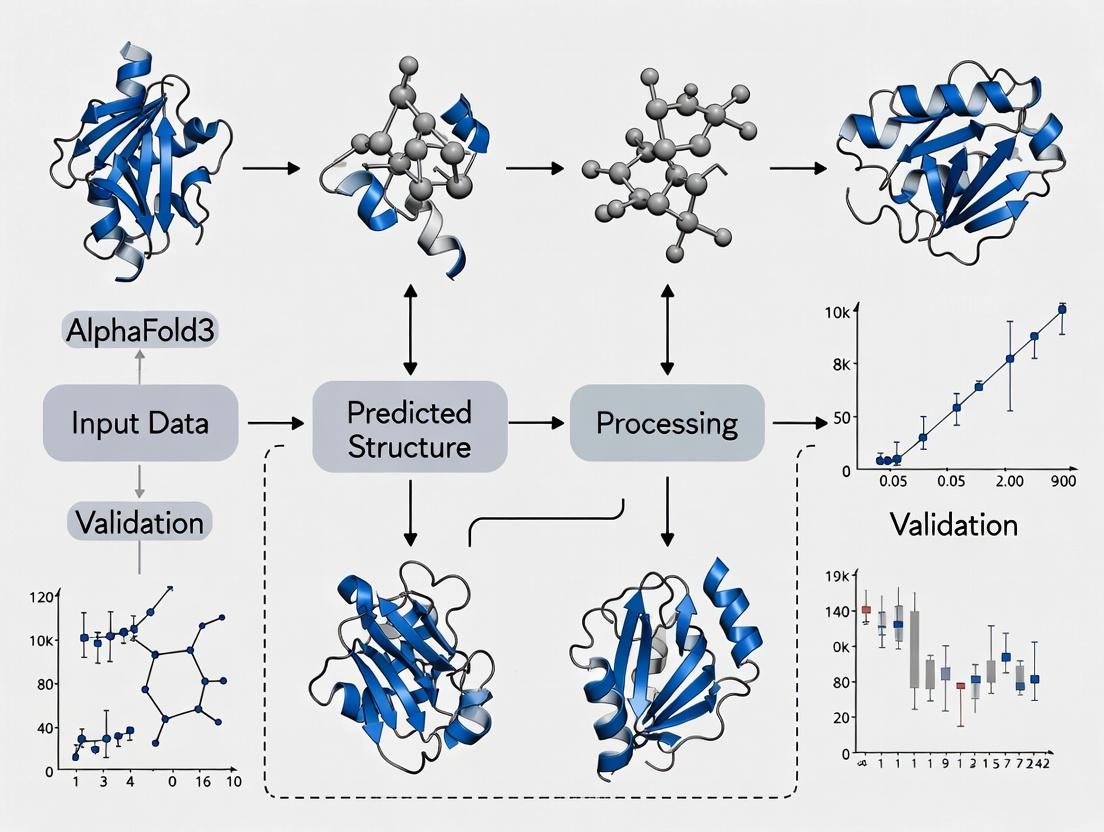
Solving Common AlphaFold3 Issues & Maximizing Prediction Accuracy
Within the broader thesis on AlphaFold3 protein structure prediction tutorial research, failed computational runs represent a significant bottleneck. These failures primarily stem from sequence-related issues, input length constraints, and server-side errors. This document provides application notes and detailed protocols to diagnose, mitigate, and resolve these common failure modes, enabling efficient research workflows for scientists and drug development professionals.
The following table categorizes common failure modes based on analysis of recent community forum reports and error logs.
Table 1: Summary of Common AlphaFold3 Run Failures and Frequencies
| Error Category | Specific Error Code/Message | Approximate Frequency* | Primary Cause |
|---|---|---|---|
| Sequence-Related | Invalid residue code (e.g., 'U', 'B', 'Z') | 35% | Non-standard amino acids in input FASTA. |
| Sequence length mismatch (multi-chain) | 15% | Inconsistent chain lengths in paired inputs. | |
| Low complexity or repetitive sequence | 20% | Sequences lacking structural diversity. | |
| Length-Related | MemoryLimitExceeded |
55% | Protein sequence or MSA depth too large for allocated RAM. |
MaxRuntimeExceeded |
40% | Total sequence length exceeding hardware/time limits. | |
GPU_OOM (Out of Memory) |
50% | Model complexity (e.g., large multimer) exhausting GPU VRAM. | |
| Server/Platform | ConnectionTimeout / APIError |
25% | Network instability or cloud service API throttling. |
DiskSpaceExceeded |
10% | Temporary file accumulation from multiple runs. | |
DependencyVersionConflict |
5% | Incompatible library versions in local installations. |
*Frequency estimates based on aggregated user reports from 2023-2024.
Experimental Protocols for Diagnosis and Mitigation
Protocol 3.1: Pre-Submission Sequence Validation and Sanitization
Objective: To ensure input protein sequences are compatible with AlphaFold3's expected alphabet and format, preventing sequence-related failures.
Materials: Raw sequence data in FASTA format, a computing environment with Python 3.9+, and the Biopython library.
Procedure:
- Install Required Tool:
pip install biopython - Execute Validation Script:
- Output: A sanitized FASTA file with non-standard residues replaced by 'X' and logged warnings.
Protocol 3.2: Systematic Length and Resource Profiling
Objective: To predict memory and runtime requirements based on sequence length, preventing hardware-related failures. Materials: Cleaned FASTA file, local AlphaFold3 installation with profiling tools. Procedure:
- Run Profiling Module: Utilize AlphaFold3's internal benchmarking script or a standalone profiler.
- Analyze Output: The script estimates peak RAM (GB), GPU VRAM (GB), and approximate runtime. Compare these values against your allocated resources (see Table 2).
- Decision Tree: If estimated requirements exceed available resources by >15%, consider (a) using a shorter construct (e.g., single domain), (b) switching to a server with higher RAM/GPU allocation, or (c) using the AlphaFold3 server API with higher-tier limits.
Table 2: Resource Benchmarks vs. Sequence Length (AlphaFold3 v3.0)
| Total Residues | Typical GPU VRAM (GB) | Typical System RAM (GB) | Avg. Runtime (CPU hrs) |
|---|---|---|---|
| < 400 | 8 - 12 | 16 - 32 | 0.5 - 1.5 |
| 400 - 800 | 12 - 20 | 32 - 64 | 1.5 - 4 |
| 800 - 1200 | 20 - 32 | 64 - 128 | 4 - 10 |
| 1200 - 2000 | 32+ | 128+ | 10+ |
Protocol 3.3: Server Error Log Analysis and Retry Strategy
Objective: To diagnose and recover from transient server and platform errors.
Materials: Error logs from the failed run (e.g., run_log.txt, cloud console logs).
Procedure:
- Log Parsing: Search for key phrases:
"ERROR","Timeout","quota","disk". - Categorize Error: Map the log message to Table 1.
- Execute Mitigated Retry:
- For
ConnectionTimeout: Implement exponential backoff in your submission script.
- For
- Document: Record the error and solution for future reference.
Visualization of Troubleshooting Workflows
Diagram Title: AlphaFold3 Run Failure Diagnosis & Resolution Workflow
The Scientist's Toolkit: Research Reagent Solutions
Table 3: Essential Tools and Resources for Robust AlphaFold3 Experimentation
| Item | Function/Description | Example/Resource Link |
|---|---|---|
| Sequence Sanitizer | Script or tool to convert non-standard amino acids (B, J, Z, U) to standard ones or 'X'. | Bio.Seq (Biopython), custom Protocol 3.1 script. |
| Complexity Predictor | Identifies low-complexity regions that may cause model confidence drops. | SEG, CAST, or hhfilter from HH-suite. |
| Resource Profiler | Estimates memory and runtime pre-submission to match hardware. | Internal profile_model.py, or derived from Table 2 benchmarks. |
| Exponential Backoff Client | Submission script with intelligent retry logic for transient network errors. | Custom wrapper function (see Protocol 3.3). |
| Local Colabfold | A faster, less resource-intensive alternative for initial screening of constructs. | Colabfold (github.com/sokrypton/ColabFold). |
| AlphaFold3 API Key | For access to managed, scalable prediction servers with defined quotas. | Google Cloud Vertex AI, Isomorphic Labs. |
| Structured Logging System | Centralized log (e.g., JSON format) of all runs, errors, and fixes for meta-analysis. | Python logging module to a shared database. |
This document serves as a comprehensive application note for a critical module within a broader thesis on AlphaFold3 Protein Structure Prediction Tutorial Research. AlphaFold3 (AF3) represents a significant advance in atomic-level structure prediction for proteins, nucleic acids, ligands, and complexes. However, its per-residue confidence metric, pLDDT (predicted Local Distance Difference Test), remains a crucial indicator of model reliability. Regions with low pLDDT (commonly <70) are considered unreliable and pose a substantial challenge for downstream applications in structural biology and drug development. This note details current strategies to interpret, refine, and validate these regions, while explicitly outlining their practical limitations.
Interpretation and Causes of Low pLDDT
Low pLDDT scores in AF3 predictions are not random errors but carry specific biological and computational implications.
Primary Causes:
- Intrinsic Disorder: Regions that are natively unstructured or contain flexible linkers.
- Conformational Dynamics: Areas involved in large-scale movements or allosteric changes not captured in a single static prediction.
- Lack of Evolutionary Information: Sparse or noisy multiple sequence alignment (MSA) coverage for the region.
- Novel Folds or Motifs: Regions with no homologous templates in the training data.
- Post-Translational Modifications or Unmodeled Ligands: Chemical states or bound molecules critical for stability but not specified in the input.
Strategic Framework and Comparative Analysis
Strategies for addressing low-confidence regions can be categorized into in silico refinement, experimental validation, and hybrid approaches. The following table summarizes key strategies, their principles, and limitations.
Table 1: Strategic Overview for Improving Low Confidence Regions
| Strategy Category | Specific Method/Tool | Principle | Key Limitation |
|---|---|---|---|
| In Silico Refinement | AlphaFold3 Self-Consistency (Multiple Seeds) | Running AF3 with different random seeds generates an ensemble; consensus regions are more reliable. | Computationally expensive; may not resolve intrinsic disorder. |
| Protein-Specific Language Models (e.g., ESMFold) | Uses protein language models trained on sequences alone, providing an orthogonal method less dependent on MSAs. | Generally lower accuracy than AF3 for high-confidence regions. | |
| Molecular Dynamics (MD) Relaxation | Uses physics-based force fields to relax steric clashes and optimize local geometry in the predicted structure. | Short simulations rarely induce large-scale refolding; force field inaccuracies. | |
| Conformational Sampling with AF2/3 | Using trimmed or modified inputs (e.g., altered MSA depth) to sample alternative conformations. | Manual, non-systematic; success is not guaranteed. | |
| Experimental Validation & Integration | Cryo-Electron Microscopy (cryo-EM) | Directly visualizes low-resolution density; flexible regions may appear as weak or absent density. | Cost, expertise, sample preparation; low-resolution for flexible loops. |
| Hydrogen-Deuterium Exchange Mass Spectrometry (HDX-MS) | Probes solvent accessibility and dynamics, directly identifying disordered or dynamic regions. | Does not provide atomic coordinates; interpretation can be complex. | |
| Nuclear Magnetic Resonance (NMR) Spectroscopy | Provides atomic-level information on dynamics and alternative conformations in solution. | Size limitations; isotope labeling required; data analysis is complex. | |
| Cross-Linking Mass Spectrometry (XL-MS) | Provides distance restraints that can guide modeling or validate contacts. | Sparse distance information; ambiguous assignments. | |
| Hybrid Modeling | Integrative / Bayesian Modeling (e.g., using BioEn, HADDOCK) | Combines computational models with experimental data (XL-MS, NMR, cryo-EM) as restraints to optimize structures. | Requires expertise in integrative modeling; dependent on experimental data quality. |
Detailed Experimental Protocols
Protocol 4.1: AlphaFold3 Self-Consistency Ensemble Analysis
Objective: To assess the robustness of a predicted model and identify consistently folded vs. highly variable regions.
- Input Preparation: Prepare your target sequence(s) in standard FASTA format.
- Multiple AF3 Runs: Execute the AF3 inference pipeline 5-10 times, each with a distinct
model_seedparameter (e.g., 0, 1, 2, 3, 4). Ensure all other input parameters (MSA, templates if used) are identical. - Structure Alignment: Superimpose all output models onto the highest average pLDDT model using a rigid-body alignment tool (e.g.,
PyMOL aligncommand, focusing on high-confidence core regions). - Consensus Analysis: Calculate the per-residue Root-Mean-Square Fluctuation (RMSF) across the aligned ensemble. Visually inspect regions with high RMSF (>2Å) and correlate with per-model pLDDT plots.
- Interpretation: Regions with low pLDDT and high ensemble RMSF are likely intrinsically disordered or dynamically unstable. Regions with low pLDDT but low ensemble RMSF may have a consistent but potentially incorrect fold.
Protocol 4.2: HDX-MS Experimental Validation of Dynamics
Objective: To obtain experimental data on backbone amide solvent accessibility and dynamics, mapping to predicted low pLDDT regions.
- Sample Preparation: Purify the protein of interest to >95% homogeneity in a suitable buffer (e.g., 20 mM phosphate, 150 mM NaCl, pH 7.0). Protein concentration should be ~10-50 µM.
- Deuterium Labeling: Dilute the protein 10-fold into a D₂O-based labeling buffer (identical pH and salt composition). Incubate at controlled temperature (e.g., 25°C) for varying time points (e.g., 10s, 1min, 10min, 1h, 4h).
- Quenching & Digestion: At each time point, quench the reaction by lowering pH to 2.5 (final concentration) and temperature to 0°C. Immediately pass the quenched sample over an immobilized pepsin column for rapid digestion (<1 min).
- LC-MS/MS Analysis: Separate peptides using a reverse-phase UHPLC system (gradient: 5-40% acetonitrile in 0.1% formic acid over 8 min, maintained at 0°C). Analyze eluted peptides via high-resolution mass spectrometry.
- Data Processing: Use specialized software (e.g., HDExaminer, DynamX) to identify peptides, calculate deuterium uptake for each time point, and map the uptake rates onto the AF3 model.
- Correlation with pLDDT: Regions with fast deuterium uptake (high dynamics) should strongly correlate with low pLDDT scores. Discrepancies (e.g., high pLDDT with fast uptake) warrant re-investigation of the model.
Visualizations
Diagram 1: Decision Workflow for Low pLDDT Regions (76 chars)
Diagram 2: Hybrid Modeling with Experimental Data (73 chars)
The Scientist's Toolkit: Research Reagent Solutions
Table 2: Essential Reagents and Materials for Key Protocols
| Item | Category | Function in Protocol | Example/Notes |
|---|---|---|---|
| Ultrapure D₂O (99.9%) | Chemical Reagent | Solvent for HDX-MS labeling; enables deuterium exchange measurement. | Must be low in pH-altering impurities. |
| Immobilized Pepsin Column | Chromatography | Provides rapid, reproducible digestion under quench conditions (low pH, 0°C) for HDX-MS. | Poroszyme immobilized pepsin cartridge. |
| Size-Exclusion Chromatography (SEC) Buffer | Buffer | For final protein purification and transfer into optimal labeling buffer for HDX-MS or Cryo-EM. | Should be volatile (e.g., ammonium acetate) for some MS/Cryo-EM applications. |
| Cross-Linking Reagent (BS³/DSS) | Chemical Probe | Creates covalent cross-links between proximal lysines in XL-MS, generating distance restraints (<30Å). | Amine-reactive, homobifunctional, membrane-impermeable. |
| Cryo-EM Grids (Quantifoil R1.2/1.3) | Consumable | Ultrathin carbon support film with holes for vitrifying protein samples for cryo-EM imaging. | Gold or copper grids; require plasma cleaning. |
| Molecular Dynamics Software (GROMACS, AMBER) | Software License | Performs energy minimization and MD relaxation on AF3 models to alleviate steric clashes. | Requires high-performance computing (HPC) resources. |
| Integrative Modeling Suite (HADDOCK) | Web Server / Software | Computationally integrates AF3 models with experimental data to generate optimized structures. | HADDOCK requires formatted restraint files (e.g., from XL-MS). |
Application Notes
Within the broader thesis on AlphaFold3 protein structure prediction tutorial research, this protocol focuses on optimizing predictions for multi-subunit complexes. AlphaFold3 represents a paradigm shift by enabling the joint prediction of proteins, nucleic acids, ligands, and post-translational modifications. However, achieving high-accuracy models for large biomolecular assemblies requires strategic input and post-prediction analysis.
Key quantitative performance metrics from recent benchmarks are summarized below:
Table 1: AlphaFold3 Performance on Complex Targets (Representative Data)
| Target Class | Example Assemblies | Predicted Interface Accuracy (pTM) | Median DockQ Score | Key Limitation |
|---|---|---|---|---|
| Protein-Protein | Heterodimeric complexes | 0.85 - 0.92 | 0.80 (High Quality) | Accuracy degrades beyond ~1,500 residues. |
| Protein-Nucleic Acid | Transcription factor-DNA | 0.78 - 0.87 | 0.65 (Medium Quality) | DNA backbone conformation variability. |
| Protein-Ligand | Kinase-inhibitor | N/A (pLDDT >85 at site) | N/A | Limited to defined set of ~100 ligand types. |
| Multi-Chain (>5) | Small ribosomal subunit | 0.70 - 0.80 | 0.50 (Acceptable) | Computationally intensive; requires partitioning. |
Table 2: Impact of Input MSAs on Complex Prediction Accuracy
| Input Strategy | Protein-protein (DockQ) | Protein-RNA (DockQ) | Computational Cost |
|---|---|---|---|
| Paired MSAs (aligned) | 0.82 | 0.72 | Very High |
| Unpaired MSAs | 0.75 | 0.64 | High |
| Single-sequence (no MSA) | 0.45 | 0.40 | Low |
Experimental Protocols
Protocol 1: Preparing Inputs for Multi-Chain Protein Complex Prediction
Objective: To generate an optimized input configuration for predicting the structure of a heterotrimeric protein complex (Chains A, B, C).
Materials:
- FASTA sequences for each chain.
- Access to AlphaFold3 via the public server or local installation.
- Multiple sequence alignment (MSA) generation tool (optional for server use).
Methodology:
- Sequence Input:
- Create a single FASTA file. For the complex, define the assembly as a single polypeptide chain using a specific linker, e.g.,
[A]:GGGSGGGSGGGS[B]:GGGSGGGSGGGS[C]. This explicitly defines the stoichiometry and order. - Alternatively, if supported by your interface, input the chains as separate molecules and define the binding pairs.
- Create a single FASTA file. For the complex, define the assembly as a single polypeptide chain using a specific linker, e.g.,
Template and MSA Strategy (for local runs):
- Paired MSA Generation (Critical): Use tools like
jackhmmerto search databases (UniRef90, MGnify) with all chain sequences simultaneously. This co-evolutionary information is crucial for interface prediction. - Template Handling: Provide known structures of individual subunits or homolog complexes as optional templates. Do not provide low-confidence templates.
- Paired MSA Generation (Critical): Use tools like
Configuration:
- Set the
model_typeparameter tocomplex. - For assemblies >1,500 residues, consider using the
relax.max_iterations=0flag to speed up initial screening. - Run a minimum of 3-5 seeds (
num_seeds=3) to assess prediction consistency, especially for flexible regions.
- Set the
Output Analysis:
- Prioritize models with high predicted interface pTM (ipTM) or complex score over high per-residue pLDDT.
- Use the predicted alignment error (PAE) matrix to validate inter-chain contacts. A low PAE (<10 Å) between two residues in different chains indicates high confidence in their spatial proximity.
Protocol 2: Integrative Modeling with Low-Confidence Predictions
Objective: To combine multiple AlphaFold3 predictions and external data to model a large assembly.
Materials:
- AlphaFold3 predictions (multiple seeds/runs).
- Cross-linking mass spectrometry (XL-MS) or cryo-EM density map data.
- Integrative modeling platform (e.g., HADDOCK, ChimeraX).
Methodology:
- Partitioned Prediction: If the full assembly fails, split it into overlapping sub-complexes (e.g., predict A-B, B-C, A-C dimers).
- Confidence Filtering: From each sub-complex run, select the top model based on ipTM.
- Data Integration:
- Format experimental constraints (e.g., from XL-MS) into distance restraints (e.g., Cβ-Cβ < 30 Å).
- Use the AlphaFold3 models as "flexible templates" in HADDOCK, with experimental restraints guiding the docking.
- Model Scoring and Selection: Score the resulting integrative models using the HADDOCK score, which balances interface energy, restraint violation, and steric clashes. Select the cluster with the best score.
Visualization
Diagram 1: Multi-Chain Prediction Workflow
Diagram 2: Integrative Modeling Logic
The Scientist's Toolkit: Research Reagent Solutions
Table 3: Essential Resources for Optimizing Complex Predictions
| Item | Function & Relevance |
|---|---|
| Paired MSA Databases (UniRef90, MGnify) | Provides co-evolutionary signals critical for accurate interface prediction in complexes. |
| AlphaFold3 ColabFold Implementation | Provides an accessible, scriptable interface for running custom complex predictions with paired MSAs. |
| ChimeraX / UCSF PyMOL | For 3D visualization, analysis of pLDDT/PAE maps, and manual model inspection/alignment. |
| HADDOCK / IMP (Integrative Modeling Platform) | Software to drive integrative modeling by combining AF3 predictions with experimental data. |
| pdb-tools / BioPython | For scripting the manipulation of input FASTA files and output PDB models (e.g., partitioning, renaming chains). |
| Cross-linking Mass Spectrometry (XL-MS) Data | Provides distance constraints to validate and guide the docking of predicted sub-complexes. |
| Local High-Performance Computing (HPC) Cluster | Essential for running large-scale predictions of multi-chain assemblies, which are computationally prohibitive on CPUs. |
Application Notes
Within the AlphaFold3 protein structure prediction tutorial research framework, handling large protein complexes (>1,500 residues) presents significant computational memory challenges. The primary bottleneck is the attention mechanism within the Evoformer and Structure Module, whose memory consumption scales quadratically with sequence length. Exceeding available GPU memory (commonly 16-48GB) leads to job termination. The following notes summarize current strategies.
Table 1: Comparative Analysis of Memory-Saving Strategies for AlphaFold3-based Prediction
| Strategy | Mechanism | Typical Memory Reduction | Key Limitation | Best Use Case |
|---|---|---|---|---|
| Chunking (MSA & Pair) | Processes sequence in blocks during attention. | 40-60% | Can slightly reduce accuracy for long-range interactions. | Single-chain proteins >2,000 residues. |
| Gradient Checkpointing | Trades compute for memory by re-calculating activations. | 25-40% | Increases runtime by ~20%. | Any large prediction when time is less critical. |
| Low-Memory Attention | Uses memory-efficient algorithms (e.g., FlashAttention). | 30-50% | Requires specific software/hardware support. | Supported implementations on newer GPUs (V100/A100+). |
| Reducing MSA Depth | Limits the number of sequences in the multiple sequence alignment. | 20-35% | Loss of co-evolutionary signal impacts accuracy. | Initial rapid screening or template-free regions. |
| CPU-Offloading | Moves less frequently used tensors to system RAM. | 15-30% | Dramatically increases runtime due to CPU-GPU transfer. | When system RAM is abundant but GPU VRAM is low. |
| Distributed Inference | Splits model across multiple GPUs (model parallelism). | Enables >5,000 residue predictions | Requires high-end multi-GPU node and technical setup. | Very large complexes (e.g., viral capsids, ribosomes). |
Experimental Protocols
Protocol 1: Implementing Chunking for AlphaFold3 Inference
This protocol details modifying inference parameters to enable chunked calculation for large protein targets.
Materials:
- Pre-trained AlphaFold3 model weights.
- Input features (MSA, templates) for the target sequence.
- Computing node with a high-memory GPU (≥24GB VRAM recommended).
Procedure:
- Feature Generation: Prepare standard input features using tools like MMseqs2 and HMMer. For sequences >2,000 residues, manually limit the MSA depth to 512 sequences to reduce initial memory load.
- Configuration Modification: Access the AlphaFold3 inference configuration file (
inference_config.yaml). Locate the parameters governing the Evoformer and Structure Module. - Set Chunking Parameters:
- Set
chunk_sizefor bothmsa_pairandpairrepresentations to a value between 128 and 256. Lower values save more memory but increase overhead. - Enable
chunkedby setting it toTrue.
- Set
- Enable Gradient Checkpointing: In the same configuration, set
gradient_checkpointing: Truefor all modules. - Run Inference: Execute the modified AlphaFold3 job. Monitor GPU memory usage via
nvidia-smi. If the job fails, reduce thechunk_sizefurther or combine with CPU-offloading for the language model embedding lookups.
Protocol 2: Distributed Inference Across Multiple GPUs
This protocol outlines a framework for predicting structures of mega-complexes using model parallelism.
Materials:
- High-performance computing cluster node with 4-8 interconnected GPUs (e.g., NVLink).
- Distributed computing library (e.g., JAX
pmap, PyTorchDistributedDataParallel). - Modified AlphaFold3 pipeline supporting model sharding.
Procedure:
- Environment Setup: Install all dependencies and ensure GPU-to-GPU communication is functional. This often requires a specific version of DeepSpeed or Horovod.
- Model Sharding Configuration: Partition the AlphaFold3 model. A common strategy is to place different blocks of the Evoformer stack on different GPUs. The Structure Module is typically kept on a primary GPU.
- Data Pipeline Modification: Implement a custom data loader that pre-splits the input features (MSA, pair representations) and broadcasts tensors to the appropriate GPUs, minimizing inter-GPU data transfer during runtime.
- Launch Inference: Use a distributed launcher (e.g.,
torchrun,mpirun) to spawn multiple processes, one per GPU. Each process loads its assigned model partition. - Synchronization & Output: Ensure synchronized communication at each attention step between shards. The final atomic coordinates and confidence metrics are collected on the master GPU/process for output in standard PDB and JSON formats.
Visualizations
Title: Decision Workflow for Large Protein Prediction
Title: Chunked Attention Mechanism for Memory Savings
The Scientist's Toolkit
Table 2: Key Research Reagent Solutions for Large-Scale AlphaFold3 Work
| Item/Reagent | Function & Application |
|---|---|
| NVIDIA A100/A800 (80GB) | High-memory GPU enabling larger chunk sizes, reducing the need for complex parallelism. |
| FlashAttention-2 Library | Integrated memory-efficient attention algorithm that reduces VRAM footprint and speeds computation. |
| ColabFold (AlphaFold3 ver.) | Provides an accessible interface with built-in memory optimizations (chunking, low-memory attention) for testing. |
| DeepSpeed Inference | Framework for easy implementation of model parallelism, CPU-offloading, and activation checkpointing. |
| JAX/PAX Framework | Native framework for AlphaFold3, allowing fine-grained control via jax.lax.scan for manual loop implementation of chunks. |
| High-Bandwidth Memory (HBM2e) | System RAM (≥512GB) used for CPU-offloading strategies to store optimizer states and large activations. |
| Slurm/CIQ Workload Manager | For orchestrating distributed multi-GPU and multi-node inference jobs on HPC clusters. |
AlphaFold3 (AF3) represents a paradigm shift in predicting biomolecular structures and interactions. However, its outputs are probabilistic, and ambiguous results—characterized by low pLDDT/ipTM scores, conformational variability, or discordance with experimental data—are common. This document provides application notes and protocols for systematically interpreting such ambiguous predictions within a research workflow.
Quantitative Metrics of Confidence in AF3
The following table summarizes AF3's key confidence metrics and their interpretation thresholds.
Table 1: Primary AlphaFold3 Confidence Metrics and Interpretive Guidelines
| Metric | Description | High Confidence Range | Low Confidence/Ambiguous Range | Recommended Action for Low Scores |
|---|---|---|---|---|
| pLDDT (per-residue) | Local Distance Difference Test. Measures local backbone reliability. | >90 (Very high) 70-90 (Confident) | 50-70 (Low) <50 (Very low) | Treat backbone geometry with skepticism. Prioritize for experimental validation. |
| ipTM (interface) | Interface Predicted TM-score. Measures confidence in protein-protein or protein-ligand interface. | >0.8 | <0.6 | Predicted interface topology is likely unreliable. |
| pTM (predicted TM-score) | Global TM-score for monomers/complexes. Measures overall fold accuracy. | >0.7 | <0.5 | The overall topology prediction may be incorrect. |
| PAE (Predicted Aligned Error) | 2D matrix estimating error (Å) in relative position of residue pairs. | Expected position error < 5Å for most pairs. | Expected position error > 10Å for many pairs. | Indicates high domain flexibility, disorder, or mis-pairing. Use to identify rigid domains vs. flexible linkers. |
Experimental Protocols for Validating Ambiguous Predictions
Protocol 3.1: In-silico Saturation Analysis for Ambiguous Binding Pockets
Purpose: To distinguish a genuine, poorly predicted ligand-binding site from a computational artifact. Methodology:
- Extract the ambiguous protein-ligand complex prediction from AF3.
- Using molecular docking software (e.g., AutoDock Vina, GNINA), prepare the protein structure, focusing on the predicted pocket.
- Generate a library of small, diverse molecular fragments (e.g., from ZINC20 fragment library).
- Dock each fragment into the pocket. Run multiple independent docking trajectories.
- Analysis: Calculate the consensus binding pose and score. A true pocket will show a favorable, convergent binding energy landscape for multiple fragments. An artifact will show no consensus and highly variable, unfavorable scores.
- Correlate findings with the AF3 ipTM and per-residue pLDDT of the pocket.
Protocol 3.2: Limited Proteolysis-Mass Spectrometry (LiP-MS) for Conformational Validation
Purpose: To experimentally probe the solvent accessibility and folding of regions predicted with low confidence. Methodology:
- Express and purify the protein of interest.
- Based on the AF3 prediction with ambiguous regions (low pLDDT), identify specific sequence segments for monitoring.
- Subject the native protein to limited proteolysis using a broad-specificity protease (e.g., proteinase K) under non-denaturing conditions for a time series (e.g., 0, 30 sec, 2, 5, 15 min).
- Quench reactions, digest to completion with trypsin, and analyze by LC-MS/MS.
- Analysis: Identify protease-accessible cleavage sites. Regions predicted with low confidence that are rapidly cleaved likely correspond to disordered or misfolded segments. Regions predicted with low confidence that are protected from cleavage may indicate a stable but difficult-to-predict fold, warranting further structural study.
Protocol 3.3: Cross-linking Mass Spectrometry (XL-MS) for Validating Ambiguous Complex Interfaces
Purpose: To obtain experimental distance restraints for protein-protein or protein-ligand interfaces with low ipTM scores. Methodology:
- Prepare the individual components of the biomolecular complex.
- Mix components under native conditions and treat with a lysine-reactive cross-linker (e.g., DSSO or BS3).
- Quench, digest, and enrich for cross-linked peptides.
- Analyze by LC-MS/MS using fragmentation methods capable of identifying cross-links (e.g., MS2-MS3).
- Analysis: Identify cross-linked residue pairs. Map these distance restraints (< 30 Å for DSSO) onto the ambiguous AF3 complex model. A model is supported if a high proportion of experimental cross-links are satisfied. Systematic violations (>25% of cross-links exceeding restraint distance) suggest the AF3 interface prediction is incorrect.
Visual Guides and Decision Frameworks
Decision Flow for Ambiguous AF3 Results
Validation Workflow for Ambiguous Regions
The Scientist's Toolkit: Research Reagent Solutions
Table 2: Essential Reagents and Resources for AlphaFold3 Validation
| Item / Resource | Function / Purpose | Example / Specification |
|---|---|---|
| AlphaFold3 Server / Local Installation | Primary prediction engine for structure/complex modeling. | Access via Google Cloud Public Preview or local ColabFold implementation with AF3 parameters. |
| ColabFold | Streamlined, accelerated pipeline for running AlphaFold, including custom MSA generation. | Essential for batch processing, sampling multiple seeds to assess model variability. |
| DSSO (Disuccinimidyl sulfoxide) | MS-cleavable cross-linker for XL-MS (Protocol 3.3). Provides distance restraints (<30Å). | Enables unambiguous identification of cross-linked peptides via MS2-MS3 fragmentation. |
| Proteinase K | Broad-specificity protease for LiP-MS (Protocol 3.2). Cleaves solvent-accessible, flexible loops. | Must be >99% pure, molecular biology grade, for controlled, limited proteolysis. |
| Fragment Library (for Docking) | Curated set of small, diverse molecules for in-silico binding site validation (Protocol 3.1). | ZINC20 Fragment Library or similar. Size: <250 Da, complying with Rule of 3. |
| Molecular Dynamics Software (e.g., GROMACS) | To assess the stability of ambiguous predicted regions via simulation. | Open-source package for simulating atomic-level dynamics; tests if a predicted fold is stable or collapses. |
| PyMOL / ChimeraX | 3D visualization software for analyzing PAE plots, pLDDT coloring, and mapping experimental data. | Critical for manual inspection and integrating validation data onto 3D models. |
Validating AlphaFold3 Predictions & Benchmarking Against AF2 and Experimental Data
Within the broader thesis on AlphaFold3 protein structure prediction tutorial research, the validation of predicted protein structures against experimentally determined Protein Data Bank (PDB) structures is a critical step. This protocol details the application of Root Mean Square Deviation (RMSD) and Global Distance Test (GDT) metrics to assess prediction accuracy, providing researchers and drug development professionals with standardized methods for benchmarking and refining computational models.
Key Metrics for Structural Validation
Root Mean Square Deviation (RMSD)
RMSD quantifies the average distance between the atoms (typically Cα atoms) of superimposed protein structures. A lower RMSD indicates higher similarity between the predicted and experimental structures.
Calculation Protocol:
- Structure Preparation: Isolate the protein chain of interest. Remove water molecules, ions, and ligands. Ensure both structures (predicted and PDB reference) contain the same number of residues for the region being compared.
- Sequence Alignment: Align the sequences of the predicted and reference structures to ensure residue correspondence. Tools like
Biopythonorclustalocan be used. - Structural Superposition: Perform a rigid-body superposition to minimize the RMSD. This involves translating and rotating the predicted structure to best fit the reference structure.
- Tool: Use
US-align,PyMOL(aligncommand), orBiopython'sSuperimposer. - Command Example (PyMOL):
align prediction, reference
- Tool: Use
- RMSD Calculation: After superposition, calculate the RMSD over the Cα atoms.
- Formula: RMSD = √[ Σ( di² ) / N ], where di is the distance between the ith pair of Cα atoms and N is the total number of atom pairs.
- Tool Output: Most superposition tools directly report the Cα RMSD.
Global Distance Test (GDT)
GDT measures the percentage of Cα atoms in the predicted model that fall within a defined distance cutoff from their corresponding positions in the reference structure, under optimal superposition. Common cutoffs are 1Å, 2Å, 4Å, and 8Å. GDTTS (Total Score) is the average of GDTP1, GDTP2, GDTP4, and GDT_P8.
Calculation Protocol:
- Preprocessing: Follow steps 1-3 from the RMSD protocol for structure preparation and initial alignment.
- Optimal Superposition for GDT: The superposition is optimized specifically to maximize the number of residues within the distance cutoffs, which may differ from the RMSD-minimizing fit.
- Distance Calculation & Percentage Analysis: For each specified cutoff distance, calculate the percentage of Cα atom pairs that are within that threshold.
- Tool: Use
TM-alignorLGA(Local-Global Alignment), which are standard for CASP assessments. - Command Example (TM-align):
TMalign prediction.pdb reference.pdb
- Tool: Use
- Score Compilation: The tool reports GDTPn scores and the composite GDTTS score.
Table 1: Interpretation of RMSD and GDT_TS Scores for Model Quality
| Metric | Score Range | Quality Interpretation | Typical Use Case |
|---|---|---|---|
| Cα RMSD | < 1.0 Å | Very High Accuracy | Near-experimental quality, reliable for detailed mechanism/docking. |
| 1.0 - 2.0 Å | High Accuracy | Excellent prediction, reliable for fold and active site analysis. | |
| 2.0 - 3.5 Å | Medium Accuracy | Correct fold, but loops/side chains may be misplaced. | |
| > 3.5 Å | Low Accuracy/Likely Incorrect Fold | Use with caution; may indicate topological errors. | |
| GDT_TS | 90 - 100 | Very High Accuracy | Near-perfect backbone alignment. |
| 70 - 90 | High Accuracy | Correct fold with minor local deviations. | |
| 50 - 70 | Medium Accuracy | Correct global fold with significant local errors. | |
| < 50 | Low Accuracy/Likely Incorrect Fold | Potential for major structural errors. |
Table 2: Comparison of Validation Tools and Their Outputs
| Tool | Primary Metric | Key Outputs | Strengths | Best For |
|---|---|---|---|---|
| PyMOL | RMSD | Cα RMSD, visual alignment. | Excellent visualization, interactive. | Quick checks, visualization, and figures. |
| TM-align | GDT_TS, TM-score | GDTHS, GDTTS, TM-score, alignment. | Fold-level assessment, alignment accuracy. | Benchmarking, CASP-style evaluation. |
| US-align | RMSD, TM-score | RMSD, TM-score, scaled scores. | Fast, scalable for large datasets. | Large-scale model validation. |
| MolProbity | Clashscore, Rotamers | All-atom contacts, rotamer outliers. | All-atom steric and dihedral validation. | Assessing atomic-level plausibility. |
Integrated Validation Workflow Protocol
This protocol describes a comprehensive validation pipeline for an AlphaFold3 prediction against a PDB structure.
Step 1: Data Retrieval and Preparation
- Input: AlphaFold3 prediction (
.pdb), PDB ID of experimental reference. - Action: Download the experimental structure from the PDB. Isolate the relevant protein chain(s) using a molecular viewer or
pdb-tools. Remove non-protein entities.
Step 2: Sequence and Length Harmonization
- Action: Align sequences using a tool like
Clustal Omega. Trim the predicted and experimental structures to include only residues that are present in both to ensure a like-for-like comparison.
Step 3: Structural Alignment and Metric Calculation
- Action (Global Fold): Run
TM-alignorUS-alignwith the trimmed structures.TMalign af_prediction_trimmed.pdb pdb_reference_trimmed.pdb
- Record: GDTTS, GDTHA, TM-score, and the resulting RMSD from this alignment.
- Action (Core Structure): Perform a strict Cα superposition in PyMOL (
align af_core, ref_core, cycles=0) to calculate the RMSD for well-aligned regions only.
Step 4: All-Atom and Steric Validation
- Action: Submit the AlphaFold3 prediction (untrimmed) to the
MolProbityweb server or usePHENIXsuite tools. - Record: Clashscore, percentage of poor rotamers, and Ramachandran outliers.
Step 5: Analysis and Reporting
- Action: Compile all metrics. Use GDT_TS/TM-score for overall fold accuracy, RMSD for local backbone precision, and MolProbity scores for model realism. Visually inspect key functional sites (e.g., active sites) in PyMOL.
Workflow and Relationship Diagrams
Title: Protein Structure Validation Workflow
Title: Relationship Between Validation Metrics
The Scientist's Toolkit: Research Reagent Solutions
Table 3: Essential Software and Resources for Structure Validation
| Item | Primary Function | Key Utility in Validation | Access Link |
|---|---|---|---|
| PyMOL | Molecular Visualization | Visual inspection, manual superposition, and RMSD calculation. | Commercial / Educational |
| ChimeraX | Molecular Visualization | Integrated superposition tools (matchmaker) and clear metric reporting. |
Free Download |
| TM-align | Structural Alignment | Calculates GDT_TS, TM-score, and optimal alignment for fold-level comparison. | Web Server / Download |
| US-align | Universal Structural Alignment | Fast, accurate alignment for protein and complex structures. | Web Server / Download |
| pdb-tools | PDB File Manipulation | Python suite for cleaning, trimming, and managing PDB files programmatically. | GitHub Repository |
| MolProbity | All-Atom Contact Analysis | Validates steric clashes, rotamer quality, and Ramachandran geometry. | Web Server |
| PDB Protein Data Bank | Experimental Structure Repository | Source of ground-truth reference structures for validation. | rcsb.org |
| AlphaFold DB | Pre-computed Predictions | Source of AlphaFold2/3 predictions for many proteins for comparison. | alphafold.ebi.ac.uk |
This document serves as an Application Note and Protocol suite within the broader thesis on AlphaFold3 protein structure prediction tutorial research. It provides a structured, technical comparison between AlphaFold2 (AF2) and AlphaFold3 (AF3), focusing on quantitative performance metrics, experimental protocols for validation, and practical toolkits for researchers in structural biology and drug development.
Quantitative Performance Comparison
The following tables summarize key performance metrics based on current benchmark data.
Table 1: Accuracy & Scope Comparison
| Metric | AlphaFold2 | AlphaFold3 | Notes |
|---|---|---|---|
| Average TM-score (Protein) | ~0.88 | ~0.90 | On CASP14 benchmark. AF3 shows modest but consistent improvement. |
| Ligand RMSD (Å) | N/A | < 1.0 | AF3 can accurately place small molecules (e.g., ions, ligands) within binding pockets. |
| Nucleotide Interface Accuracy | Not Applicable | ~90% | AF3 predicts protein-DNA/RNA interfaces with high confidence. |
| Antibody Paratope Prediction | Low Accuracy | ~40% Improvement | AF3 significantly better at modeling antibody-antigen interfaces. |
| Multimer Modeling (DockQ) | ~0.60 | ~0.72 | AF3 shows major improvement in protein-protein complex prediction quality. |
Table 2: Computational Performance
| Metric | AlphaFold2 | AlphaFold3 | Notes |
|---|---|---|---|
| Model Parameters | ~93 million | ~??? million | AF3 architecture (Diffusion) is fundamentally different; exact size not publicly detailed. |
| Typical Runtime (Single Chain) | Minutes to Hours (GPU) | Reportedly Faster | AF3's diffusion-based approach is cited as more computationally efficient for certain tasks. |
| Hardware Requirement | High (GPU + High RAM) | Similar / Optimized | Both require significant GPU memory for full models; AF3 available primarily via cloud API. |
| Access Mode | Open Source (Local) | Cloud API Only | Critical difference. AF2 is freely installable; AF3 is accessed via the AlphaFold Server. |
Experimental Protocols for Validation
Protocol 3.1: Benchmarking Predicted Protein-Ligand Complexes against Experimental Structures
- Objective: Quantitatively assess the accuracy of AF3's ligand placement predictions.
- Materials: AlphaFold Server access, PDB structures with bound ligands (e.g., ATP, heme, drug molecules), visualization software (PyMOL, ChimeraX), computational geometry tools (OpenBabel, RDKit).
- Procedure:
- Target Selection: Curate a set of protein-ligand complexes from the PDB. Ensure experimental resolution is < 2.5 Å.
- Input Preparation: For each target, submit the protein sequence and the ligand SMILES string to the AlphaFold Server via its interface.
- Prediction Execution: Run AF3 prediction with default settings. Download the predicted model in PDB format.
- Structural Alignment: Superimpose the predicted protein structure onto the experimental protein backbone (from the PDB) using PyMOL's
aligncommand. - Ligand RMSD Calculation: Isolate the predicted ligand and the experimental ligand coordinates. Calculate the Root-Mean-Square Deviation (RMSD) of the heavy atoms after the protein superposition.
- Analysis: A ligand RMSD < 1.0 Å indicates high-accuracy placement. Compare success rates across different ligand classes.
Protocol 3.2: Evaluating Protein-Protein Complex (Multimer) Predictions
- Objective: Validate the improvement of AF3 in modeling protein-protein interactions.
- Materials: AlphaFold2 (local install), AlphaFold Server, benchmark dataset (e.g., Dockground), DockQ scoring software.
- Procedure:
- Dataset Preparation: Compile a list of known binary protein complexes with available experimental structures. Provide sequences for both partners.
- Parallel Prediction: For each complex:
- Run AF2-Multimer v2.3.1 locally using the standard multimer inference pipeline.
- Submit the two sequences to the AlphaFold Server for complex prediction.
- Scoring: For both the AF2 and AF3 outputs, calculate the DockQ score using the official DockQ program against the experimental reference structure.
- Classification: Use DockQ scores to classify predictions as High (DockQ ≥ 0.8), Medium (0.8 > DockQ ≥ 0.5), or Low (DockQ < 0.5) quality. Tabulate the percentage of predictions in each category for AF2 vs. AF3.
Visualizations: Workflow & Architecture
Title: AF2 vs AF3 Prediction Workflow Divergence
Title: Model Validation & Scoring Protocol
The Scientist's Toolkit: Research Reagent Solutions
Table 3: Essential Resources for AlphaFold-Based Research
| Item | Function | Example / Source |
|---|---|---|
| AlphaFold2 Local Installation | Provides full control, batch processing, and customization for protein-only predictions. | GitHub: google-deepmind/alphafold |
| AlphaFold Server Access | Essential for accessing AlphaFold3 capabilities, including ligand and nucleic acid modeling. | alphafoldserver.com |
| Structural Biology Database | Source of experimental structures for benchmark datasets and input templates (disabled in AF3). | Protein Data Bank (PDB) |
| Visualization & Analysis Software | For visualizing predicted models, calculating metrics, and preparing figures. | PyMOL, UCSF ChimeraX, BIOVIA Discovery Studio |
| DockQ Scoring Software | Standardized tool for evaluating the quality of protein-protein complex predictions. | GitHub: bjornwallner/DockQ |
| Chemical Format Toolkits | Converts and processes ligand SMILES strings for input and RMSD analysis. | RDKit, OpenBabel |
Within a broader thesis on AlphaFold3 protein structure prediction tutorial research, benchmarking against empirical structural biology techniques is essential. AlphaFold3's predictions of protein structures, complexes, and modifications must be validated against the gold-standard experimental methods: Cryo-Electron Microscopy (Cryo-EM), X-ray Crystallography, and Nuclear Magnetic Resonance (NMR) spectroscopy. This application note details protocols for experimental structure determination and provides a framework for comparative analysis with computational predictions.
Table 1: Comparison of Key Structural Biology Techniques
| Parameter | X-ray Crystallography | Cryo-EM (Single Particle Analysis) | NMR Spectroscopy | AlphaFold3 Prediction |
|---|---|---|---|---|
| Typical Resolution Range | 1.0 - 3.5 Å | 1.8 - 4.5 Å (for well-behaved samples) | Not directly comparable; ensemble of structures | Reported accuracy (pLDDT) correlates with ~1-5 Å local accuracy |
| Optimal Sample Size (mg) | 5-20 mg (for screening) | 0.1-0.5 mg (at ~1-3 mg/mL) | 5-20 mg (isotopically labeled) | N/A (in silico) |
| Typical Time to Structure | Weeks to years | Days to months (post-grid prep) | Months to years | Minutes to hours |
| Size Range (kDa) | No strict upper limit; diffusion may limit very large crystals | >50 kDa (optimal); smaller possible with symmetry | <50 kDa (optimal in solution) | Theoretically unlimited; performance varies |
| Sample State | Crystalline solid | Vitrified solution (frozen-hydrated) | Solution (native conditions) | N/A |
| Key Output Metric | Electron density map | 3D Coulomb potential map | Ensemble of models & restraint data | Predicted model with per-residue pLDDT & predicted aligned error (PAE) |
| Information on Dynamics | Limited (B-factors) | Limited (flexibility from heterogeneous refinement) | Atomic-level dynamics (ps-ns timescale) | Limited (confidence metrics may infer flexibility) |
Application Notes & Protocols
Protocol 1: Cryo-EM Single Particle Analysis Workflow for Validation of a Large Protein Complex
Objective: Determine a sub-3 Å resolution structure of a ~500 kDa protein complex to validate an AlphaFold3 multimer prediction.
Research Reagent Solutions & Key Materials:
- Purified Protein Complex (>0.5 mg/mL): High-purity, monodisperse sample in suitable buffer (e.g., HEPES, Tris).
- Quantifoil R1.2/1.3 or R2/2 300-mesh Au Grids: Conductance grids for optimal ice thickness.
- Liquid Ethane/Propane Mix: Cryogen for rapid vitrification.
- Vitrobot Mark IV (Thermo Fisher) or equivalent: Automated plunge freezer for reproducible grid preparation.
- 300 keV Cryo-TEM (e.g., Titan Krios, Glacios): High-end electron microscope equipped with a direct electron detector (e.g., Gatan K3, Falcon 4).
- Processing Software Suite (RELION, cryoSPARC, cisTEM): For computational reconstruction.
Detailed Methodology:
- Grid Preparation & Vitrification:
- Apply 3-4 µL of protein sample to a glow-discharged grid.
- Blot for 2-6 seconds at 100% humidity, 4°C, then plunge into liquid ethane.
- Store grids in liquid nitrogen.
Screening & Data Collection:
- Screen grids for ice quality and particle distribution.
- Collect a dataset of 5,000-10,000 movies at a nominal magnification of 105,000x (0.825 Å/pixel), with a total electron dose of 40-60 e⁻/Ų, fractionated over 40-50 frames.
Image Processing & Reconstruction (cryoSPARC v4 workflow):
- Patch Motion Correction & CTF Estimation: Correct for beam-induced motion and estimate contrast transfer function per micrograph.
- Particle Picking: Use template picker or Topaz to extract ~1-2 million particle images.
- 2D Classification: Remove junk particles by selecting classes with high-resolution features.
- Ab-initio Reconstruction & Heterogeneous Refinement: Generate 3-4 initial models to remove compositional heterogeneity.
- Non-uniform Refinement: Refine the final set of particles to obtain a high-resolution map. Apply post-processing (masking, B-factor sharpening) to estimate final resolution via Fourier Shell Correlation (FSC=0.143).
Model Building & Refinement:
- Fit the AlphaFold3 predicted model into the cryo-EM density map using ChimeraX or Coot.
- Manually correct regions with poor fit and refine using real-space refinement in Phenix.
Protocol 2: High-Resolution X-ray Crystallography for a Small Protein Target
Objective: Solve a 1.5 Å crystal structure of a 25 kDa protein for atomic-level validation of AlphaFold3 side-chain packing predictions.
Research Reagent Solutions & Key Materials:
- Crystallization Screen Kits (e.g., JCSG+, Morpheus, PEG/Ion): Sparse matrix screens for initial condition identification.
- Sitting-Drop Vapor Diffusion Plates (96-well): Standard for high-throughput crystallization trials.
- Liquid Nitrogen Dewar: For crystal cryo-cooling and storage.
- Synchrotron Beamline Access: Source of high-intensity X-rays (e.g., Diamond Light Source, ESRF).
- Data Processing Suite (XDS, DIALS, HKL-2000): For indexing, integration, and scaling.
- Phasing & Refinement Software (PHASER, phenix.refine, Refmac):
Detailed Methodology:
- Crystallization:
- Set up 96-well sitting-drop plates using a liquid handling robot. Mix 100 nL protein (10-20 mg/mL) with 100 nL reservoir solution.
- Incubate at 293K. Identify hits within 1-14 days.
- Optimize hits manually using hanging-drop vapor diffusion in 24-well plates.
Cryo-protection & Data Collection:
- Soak crystal in reservoir solution supplemented with 20-25% glycerol or ethylene glycol.
- Mount crystal on a nylon loop and flash-cool in liquid nitrogen.
- Collect a 360° dataset at 100K on a synchrotron microfocus beamline with a Pilatus 6M detector. Aim for high multiplicity (>5) and completeness (>99%).
Data Processing, Phasing & Refinement:
- Process data: index, integrate, and scale using XDS and AIMLESS.
- Perform molecular replacement using the AlphaFold3 predicted model as a search model in PHASER.
- Run iterative cycles of manual model building in Coot and refinement in phenix.refine (using TLS, occupancy, and individual B-factor parameters).
- Validate final model with MolProbity.
Protocol 3: NMR Spectroscopy for Dynamics and Validation in Solution
Objective: Obtain chemical shift assignments and residual dipolar coupling (RDC) data for a 15 kDa protein to validate the conformational ensemble predicted by AlphaFold3.
Research Reagent Solutions & Key Materials:
- Uniformly ¹⁵N/¹³C-Labeled Protein Sample: Produced via bacterial expression in M9 minimal media with ¹⁵NH₄Cl and ¹³C-glucose.
- NMR Buffer (e.g., 20 mM Phosphate, 50 mM NaCl, pH 6.8, 10% D₂O): For stable, aggregation-free samples.
- 5 mm NMR Tubes: Shigemi or equivalent for minimal sample volume.
- High-Field NMR Spectrometer (≥600 MHz, Cryoprobe-equipped): For high-sensitivity data acquisition.
- Alignment Media (e.g., Pf1 Phage, PEG/Hexanol): To induce partial alignment for RDC measurements.
- Processing/Assignment Software (NMRPipe, NMRFAM-SPARKY, CCPNmr Analysis):
Detailed Methodology:
- Sample Preparation:
- Prepare ~0.3 mL of 0.5-1.0 mM uniformly labeled protein in NMR buffer.
- For RDCs, add alignment media to achieve a ²H splitting of 10-30 Hz.
NMR Experiments & Data Collection:
- At 298K, collect a suite of 2D/3D experiments for backbone and side-chain assignment: ¹H-¹⁵N HSQC, HNCA, HNCOCA, HNCACB, CBCACONH.
- Collect ¹H-¹⁵N RDC data by comparing ¹H-¹⁵N HSQC spectra of aligned and isotropic samples.
Data Processing & Analysis:
- Process all data with NMRPipe. Use NMRFAM-SPARKY for peak picking and assignment.
- Assign backbone chemical shifts using CARA or PINE.
- Calculate RDCs from peak position differences.
- Validate the AlphaFold3 model by back-calculating chemical shifts (via SHIFTX2) and RDCs (from structural tensor alignment in PALES) and comparing to experimental data.
Visualization of Methodologies and Relationships
Title: AlphaFold3 Validation Workflow Against Experiments
Title: Technique Comparison for Benchmarking
The Scientist's Toolkit: Essential Reagents & Materials
Table 2: Key Research Reagent Solutions for Structural Validation
| Item | Function in Context | Example/Note |
|---|---|---|
| HEPES/Tris Buffer Systems | Maintains protein stability and pH during purification, grid preparation, and crystallization. | 20-50 mM, pH 7.0-8.5, often with 100-300 mM NaCl. |
| PEG-based Crystallization Screens | Precipitants that drive protein solution to supersaturation, promoting crystal nucleation and growth. | JCSG+, PEG/Ion, Morpheus screens. PEG size/concentration is key variable. |
| Quantifoil or UltrAuFoil Grids | Cryo-EM support films with patterned holes, enabling consistent vitrification over holes for imaging. | Au grids (300 mesh) are standard. R1.2/1.3 (1 µm holes) common. |
| Liquid Ethane (Propane Mix) | Cryogen with high heat capacity for rapid vitrification of aqueous samples, forming amorphous, non-crystalline ice. | Essential for preserving high-resolution sample details in Cryo-EM. |
| Cryo-Protectants (Glycerol, MPD) | Displace water to prevent crystalline ice formation during cryo-cooling of crystals for X-ray diffraction. | Typically 15-25% v/v. Soak time is critical to avoid crystal damage. |
| Isotopically Labeled Nutrients (¹⁵NH₄Cl, ¹³C-Glucose) | Enables isotopic labeling of proteins for NMR spectroscopy, allowing detection of backbone and side-chain nuclei. | Required for multi-dimensional NMR experiments on proteins >10 kDa. |
| Pf1 Phage Alignment Media | Introduces weak, tunable anisotropic alignment for NMR samples, enabling measurement of Residual Dipolar Couplings (RDCs). | Provides long-range structural restraints for validation. |
| Direct Electron Detectors (Gatan K3, Falcon 4) | Cameras for Cryo-EM with high detective quantum efficiency (DQE) and fast readout, enabling dose-fractionated movie collection. | Revolutionized Cryo-EM resolution. |
| Synchrotron Beamtime | Provides high-flux, tunable X-rays for diffraction data collection, enabling rapid, high-resolution data acquisition. | Microfocus beams are essential for small crystals. |
| Processing Software Licenses (RELION, cryoSPARC, Phenix, CCPNmr) | Computational suites for data processing, reconstruction, model building, refinement, and analysis. | Often institutionally licensed. cryoSPARC offers on-demand licensing. |
Assessing Novel Protein and Complex Predictions in the Absence of Experimental Data
The revolutionary ability of AlphaFold3 to predict the structure of proteins and their complexes with high accuracy presents a new paradigm in structural biology. However, a critical challenge remains: how to rigorously assess the quality of these predictions when no experimental structural data exists for validation. This application note, framed within a broader thesis on AlphaFold3 methodologies, provides detailed protocols and frameworks for evaluating novel predictions, enabling researchers and drug developers to gauge reliability and prioritize targets for downstream experimental validation.
Quantitative Assessment Metrics and Benchmarks
The following metrics, derived from analysis of AlphaFold3 performance on known structures and simulated "novel" targets, provide benchmarks for evaluating novel predictions.
Table 1: Key Quantitative Metrics for AlphaFold3 Prediction Assessment
| Metric | Description | Typical Range (High Confidence) | Interpretation Guideline |
|---|---|---|---|
| Predicted Aligned Error (PAE) | Expected positional error (Å) between residues. | < 10 Å for majority of pairs. | Low PAE across complex indicates rigid, confident interaction. |
| pLDDT (per-residue) | Local Distance Difference Test; confidence score (0-100). | > 90 (Very High), 70-90 (Confident). | Residues with pLDDT < 70 may be disordered or uncertain. |
| pTM (predicted TM-score) | Global confidence metric for monomer (0-1). | > 0.7 (Good fold), > 0.8 (High accuracy). | Estimates overall topological correctness. |
| ipTM (interface pTM) | Confidence metric for complex interfaces (0-1). | > 0.8 (High confidence interface). | Primary metric for assessing complex prediction reliability. |
| Predicted DockQ Score | Estimates quality of protein-protein docking (0-1). | > 0.8 (High), 0.7-0.8 (Medium). | Useful for protein-protein complexes. |
| pLDDT Multimer | pLDDT adapted for multimeric chains. | > 85 (High confidence). | Assesses per-chain confidence in multimer context. |
Table 2: Composite Confidence Tiers for Novel Predictions
| Confidence Tier | ipTM | pLDDT (Avg. Core) | Recommended Action |
|---|---|---|---|
| Tier 1: High | ≥ 0.80 | ≥ 85 | Suitable for detailed mechanistic analysis, virtual screening. |
| Tier 2: Medium | 0.60 - 0.79 | 70 - 84 | Requires cautious interpretation; prioritize mutagenesis validation. |
| Tier 3: Low | < 0.60 | < 70 | Treat as hypothetical; requires experimental structure determination. |
Protocol: Systematic Workflow for Assessing Novel AlphaFold3 Predictions
Protocol 1: Initial Quality Control and Plausibility Check
Objective: To perform a first-pass assessment of a novel AlphaFold3 prediction for a protein complex.
Materials & Software:
- AlphaFold3 prediction output (PDB file, PAE JSON, confidence scores).
- Visualization software (e.g., PyMOL, UCSC ChimeraX).
- Bioinformatics tools (HMMER, DALI, or Foldseek servers).
Procedure:
- Load and Visualize: Load the predicted PDB file into visualization software. Color the model by pLDDT (rainbow scale: blue=high, red=low).
- Core Confidence Identification: Identify the structural core as contiguous regions with pLDDT > 80. Note any large, functionally relevant regions (e.g., active sites, binding grooves) with low confidence.
- Interface Inspection: For complexes, visually inspect the predicted interface. Ensure side chains are interdigitated, not clashing, and that polar interactions (H-bonds, salt bridges) are plausible.
- PAE Analysis: Generate and analyze the PAE plot. A "block-like" pattern along the diagonal for the complex indicates well-defined relative positioning between subunits.
- Fold Conservation Check: Submit the monomer sequence(s) to a remote homology detection server (e.g., HMMER against Pfam) or a fold comparison server (e.g., DALI Lite, Foldseek). A match to a known fold family, even with low sequence identity (<20%), increases plausibility.
Protocol 2: In silico Mutagenesis and Binding Affinity Corroboration
Objective: To computationally test the robustness of a predicted protein-ligand or protein-protein interface.
Materials & Software:
- Structure from Protocol 1.
- Computational docking software (e.g., AutoDock Vina, HADDOCK).
- Molecular dynamics setup (e.g., GROMACS, AMBER) - optional for advanced users.
Procedure:
- Conservation Analysis: Align homologs of the target protein. Map conserved residues onto the predicted structure. High confidence interfaces should be enriched in evolutionarily conserved residues.
- In silico Alanine Scanning: a. Using a computational tool like FoldX, Rosetta, or HADDOCK, perform a virtual alanine scan on interface residues. b. Calculate the predicted change in binding free energy (ΔΔG) for each mutation. c. A predicted interface is more credible if mutations to alanine at conserved, buried polar residues yield large, unfavorable ΔΔG values (> 2 kcal/mol).
- Independent Docking Validation (for protein-ligand): a. Separate the predicted ligand from the AlphaFold3 model. b. Using standard docking software (AutoDock Vina), re-dock the ligand into the predicted binding pocket without using the AF3 pose as a guide. c. A credible prediction is supported if the top-scoring independent docking pose closely aligns (RMSD < 2.0 Å) with the original AF3 prediction.
The Scientist's Toolkit: Research Reagent Solutions
Table 3: Essential Tools for Assessing Novel AlphaFold3 Predictions
| Item | Function & Relevance |
|---|---|
| AlphaFold3 Colab Notebook / Local Install | The primary engine for generating predictions. Requires proper hardware (GPU) and sequence input. |
| ChimeraX / PyMOL | For 3D visualization, coloring by confidence metrics, measuring distances, and preparing publication figures. |
| Foldseek Server | Rapidly search the predicted structure against the PDB to find distant structural homologs, providing evolutionary context. |
| HMMER Web Server | Perform sensitive sequence profile searches against databases like Pfam to identify functional domains, even in novel folds. |
| FoldX Suite | Perform quick energy calculations, alanine scanning, and stability assessments on predicted models. |
| PISA (Proteins, Interfaces, Structures and Assemblies) | Analyze protein interfaces in complexes, calculating buried surface area and solvation free energy. |
| CONCOORD / FRODAN | Generate ensembles of plausible alternative conformations to assess the rigidity/flexibility of low-confidence regions. |
| Phenix.Validate | Comprehensive validation suite; use molprobity and geometry modules to check stereochemical quality of the de novo model. |
Visualization Diagrams
Diagram 1 Title: Novel AF3 Prediction Assessment Protocol
Diagram 2 Title: Relationship of Key AF3 Confidence Metrics
1. Introduction: Context within AlphaFold3 Research AlphaFold3 represents a transformative advance in predicting the structure of proteins and their complexes with other biomolecules. However, its application in rigorous scientific and drug discovery contexts necessitates a clear, quantified understanding of its limitations. This document provides application notes and protocols for critically assessing model confidence and error margins, framing these analyses as essential components of any research workflow employing AlphaFold3 predictions.
2. Quantitative Summary of Known Limitations The performance of AlphaFold3 is not uniform across all biological contexts. Key quantitative limitations are summarized below.
Table 1: AlphaFold3 Performance Metrics and Key Limitations
| Assessment Metric / Context | Typical Performance / Limitation | Implications for Research |
|---|---|---|
| Per-Residue Confidence (pLDDT/iptm) | pLDDT > 90 (Very High), 70-90 (Confident), 50-70 (Low), <50 (Very Low). Interface pTM (iptm) for complexes. | Low-confidence regions (pLDDT<70) are potentially unstructured or mis-folded; should not be used for detailed mechanistic insight. |
| Protein-Small Molecule Ligands | Limited by training data diversity; accuracy degrades for novel chemotypes or covalent inhibitors. | Predictions of binding pose for non-canonical ligands require experimental validation. |
| Protein-Nucleic Acid Complexes | Generally high accuracy for DNA/RNA backbone, but sequence-specific contact confidence can vary. | Specific hydrogen bonding networks may be ambiguous. |
| Large Multi-Protein Assemblies | Performance decreases with increasing number of chains due to combinatorial complexity. | Global architecture may be correct, but local interfaces may be unreliable. |
| Conformational Dynamics & Flexibility | Predicts a single, static conformation. Poor at capturing multiple biologically relevant states (e.g., apo vs. holo). | Cannot model allosteric transitions, induced fit, or dynamic loops from a single prediction. |
| Antibody-Antigen Prediction | CDR loop accuracy can be variable; antigen-binding orientation may have high error margins. | Critical for therapeutic antibody development; requires cross-validation. |
| Impact of Multiple Sequence Alignment (MSA) Depth | Accuracy strongly correlates with depth and diversity of homologous sequences in the input MSA. | Targets with few homologs ("orphan" proteins) will have higher expected error. |
3. Experimental Protocols for Validation
Protocol 3.1: Systematic Analysis of Prediction Confidence Objective: To map local and global error estimates onto an AlphaFold3 prediction for targeted experimental design. Materials: AlphaFold3 prediction output (PDB file, confidence scores JSON), visualization software (PyMOL, ChimeraX). Procedure:
- Load and Color by pLDDT: Import the predicted PDB file into visualization software. Color the structure according to the per-residue pLDDT score (e.g., blue (high) -> red (low)).
- Identify Low-Confidence Regions: Isolate all residues with pLDDT < 70. Calculate the solvent-accessible surface area (SASA) of these regions. Buried low-confidence cores are a major red flag.
- Interface Analysis: For complexes, extract the interface pTM (iptm) score. Visualize and list all residues at the interface between molecules. Cross-reference with the per-residue confidence scores at the interface.
- Generate Report: Document regions requiring validation (e.g., low-confidence loops, ambiguous ligand poses, uncertain interface contacts).
Protocol 3.2: Cross-Validation with Orthogonal Biophysical Methods Objective: To empirically validate or refute specific aspects of an AlphaFold3 prediction. Materials: Purified protein/target complex, appropriate assay reagents. Procedure A (Site-Directed Mutagenesis for Interfaces):
- Based on AlphaFold3-predicted critical interface residues (both high and medium confidence), design point mutations (e.g., alanine substitutions).
- Express and purify wild-type and mutant proteins.
- Measure binding affinity (e.g., via Surface Plasmon Resonance (SPR) or ITC) for the complex.
- Interpretation: A severe drop in affinity for mutation of a predicted critical residue supports the model. Lack of effect challenges the predicted interface geometry.
Procedure B (Ligand Docking & Competition Assay):
- Using the AlphaFold3-predicted protein structure with a co-predicted small molecule, perform in silico docking of a known active and inactive analog.
- Establish a functional biochemical assay (e.g., enzymatic inhibition).
- Test the ability of the docked compounds to compete with a known reporter ligand or substrate.
- Interpretation: Correlation between predicted docking pose/scores and experimental inhibitory potency supports the accuracy of the predicted binding pocket.
4. Visualization of Analysis Workflows
Title: AlphaFold3 Critical Analysis and Validation Workflow
5. The Scientist's Toolkit: Key Research Reagents & Materials
Table 2: Essential Reagents for Validating AlphaFold3 Predictions
| Item / Solution | Function / Application in Validation |
|---|---|
| Site-Directed Mutagenesis Kit | To introduce point mutations at predicted critical residues for functional testing of interfaces or active sites. |
| Surface Plasmon Resonance (SPR) Chip & Buffers | For label-free, quantitative measurement of binding kinetics (KD, ka, kd) between predicted interacting partners. |
| Isothermal Titration Calorimetry (ITC) Kit | To measure the thermodynamic parameters (ΔH, ΔS, KD) of a binding interaction, providing high-quality binding affinity data. |
| Hydrogen-Deuterium Exchange Mass Spectrometry (HDX-MS) | To probe protein solvent accessibility and dynamics. Can validate predicted structured vs. flexible regions and binding interfaces. |
| Cryo-EM Grids & Vitrification System | For high-resolution structural validation of large complexes or conformations predicted by AlphaFold3. |
| Synchrotron Beamtime / X-ray Crystallography Plates | For obtaining atomic-resolution experimental structures to serve as ground truth for comparison. |
| Biochemical Assay Kits (e.g., Enzyme Activity) | To functionally test predictions involving catalytic activity or ligand binding via competition assays. |
| Stable Cell Line for Protein Expression | To produce high-quality, post-translationally modified protein samples that match the biological context of the prediction. |
Conclusion
AlphaFold3 represents a paradigm shift, making highly accurate structure prediction for a vast array of biomolecular systems accessible to researchers. By mastering the foundational concepts, following a rigorous methodological workflow, applying troubleshooting techniques, and critically validating outputs, scientists can reliably integrate this tool into their research pipeline. The implications are profound, promising to accelerate drug discovery by rapidly generating structural hypotheses for novel targets, protein-protein interactions, and ligand binding sites. Future directions will involve tighter integration with molecular dynamics for flexibility, direct application in rational drug design software, and the community-driven challenge of experimentally verifying the flood of novel predictions, ultimately bridging computational prediction and clinical translation.