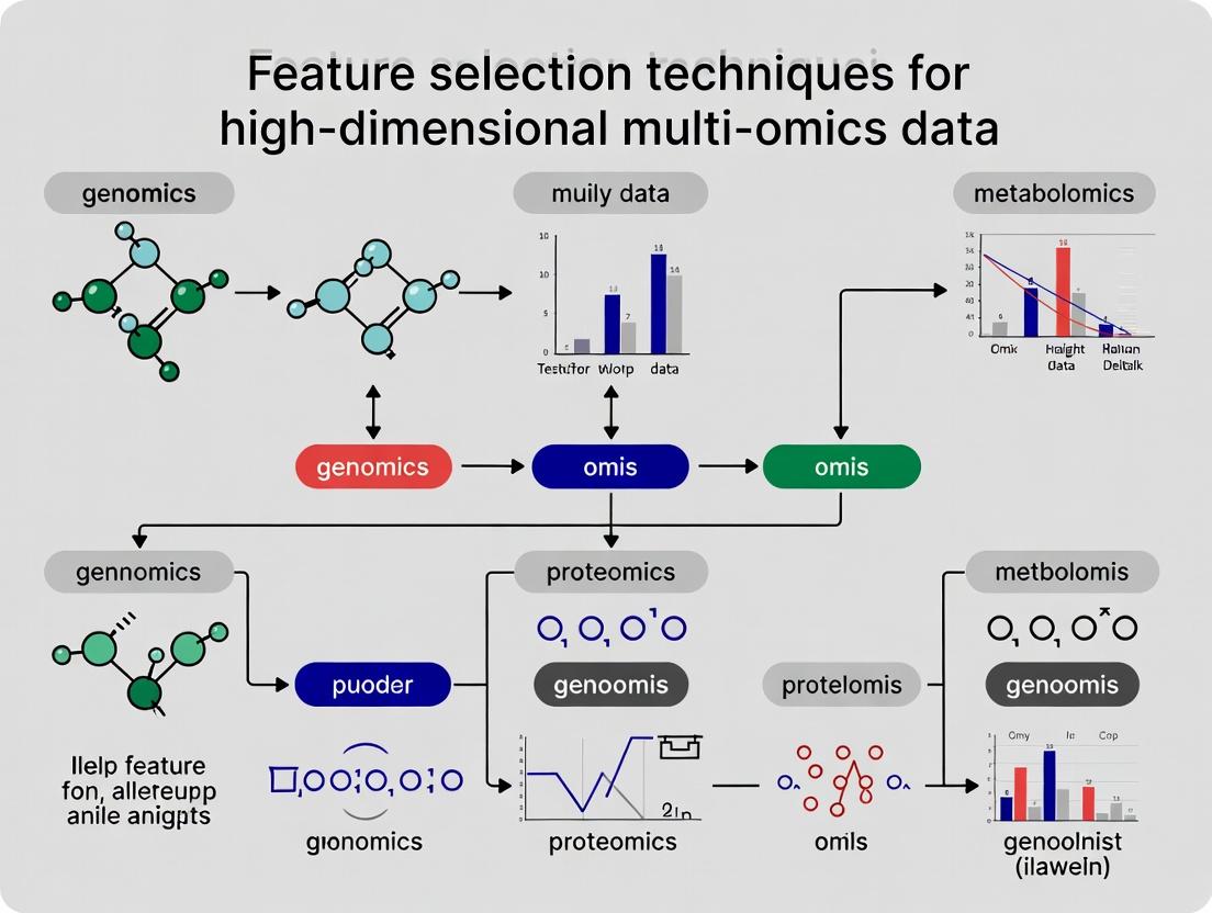
Navigating the Complexity: A Practical Guide to Feature Selection in High-Dimensional Multi-Omics Data
This comprehensive guide addresses the critical challenge of feature selection in high-dimensional multi-omics datasets, which are foundational to modern biomedical research and drug discovery.
Navigating the Complexity: A Practical Guide to Feature Selection in High-Dimensional Multi-Omics Data
Abstract
This comprehensive guide addresses the critical challenge of feature selection in high-dimensional multi-omics datasets, which are foundational to modern biomedical research and drug discovery. We first establish the nature of the 'curse of dimensionality' and the distinct characteristics of genomics, transcriptomics, proteomics, and metabolomics data. The core of the article systematically details and compares state-of-the-art methodologies, including filter, wrapper, and embedded techniques, alongside sophisticated hybrid and ensemble approaches. We provide actionable strategies for troubleshooting common pitfalls like overfitting, computational bottlenecks, and batch effects. Finally, we present a rigorous framework for validating and comparing selected features using biological databases, statistical benchmarks, and performance metrics in predictive models. This guide equips researchers with the knowledge to extract robust, biologically meaningful signals from complex, multi-layered biological data.
Understanding the Multi-Omics Landscape: What Makes Feature Selection So Crucial?
Defining the 'Curse of Dimensionality' in a Biological Context
Technical Support Center: Troubleshooting High-Dimensional Omics Analysis
Frequently Asked Questions (FAQs)
Q1: During my single-cell RNA-seq analysis, my clustering results become unstable and meaningless when I include all 20,000+ detected genes. What is happening and how can I fix it? A1: You are directly experiencing the Curse of Dimensionality. In high-dimensional spaces (like 20,000-dimensional gene expression space), distances between data points become uniformly large and similar, causing clustering algorithms to fail. To resolve this:
- Apply a robust feature selection method before clustering.
- Follow Protocol A: Variance-Stabilizing Feature Pre-Filtering (detailed below).
- Use the provided Research Reagent Solutions table for recommended tools.
Q2: My classifier trained on proteomics data shows 99% accuracy during training but performs at ~50% (random chance) on the independent validation set. What is the cause? A2: This is a classic symptom of overfitting due to high dimensionality (p >> n problem), where the number of features (p, proteins) vastly exceeds the number of samples (n). The model memorizes noise. The solution involves:
- Implementing rigorous feature selection embedded within cross-validation.
- Applying Protocol B: Nested Cross-Validation for Dimensionality-Reduced Classifier Training.
- Ensuring your training set is not used for feature selection.
Q3: When I try to visualize my multi-omics data integration results in 2D or 3D using t-SNE or UMAP, the structure looks overly "compressed" or forms artificial clusters. Why? A3: These nonlinear dimensionality reduction techniques are sensitive to the Curse. Distortions occur when trying to project from very high-dimensional spaces where local distance relationships are already unreliable. Troubleshoot by:
- Pre-processing with linear techniques (e.g., PCA) to reduce to an intermediate dimension (50-100).
- Following the Multi-Omics Dimensionality Reduction Workflow diagram.
- Systematically varying perplexity (t-SNE) or n_neighbors (UMAP) parameters.
Troubleshooting Guides
Issue: Poor Model Generalization (Overfitting)
- Symptoms: High training accuracy, low test/validation accuracy.
- Root Cause (Biological Context): In genomics, the number of potential features (genes, SNPs, methylation sites) is orders of magnitude larger than available patient samples. Random correlations between features and the outcome arise, misleading the model.
- Step-by-Step Solution:
- Identify: Split your data into Training, Validation, and Hold-out Test sets. Never use the test set until the final evaluation.
- Contain: Perform feature selection only on the training set. Use univariate statistical tests (e.g., ANOVA, chi-squared) or model-based importance.
- Validate: Train your model on the selected features from the training set. Evaluate performance on the validation set.
- Iterate: Use the validation set performance to tune the number of features selected.
- Finalize: Retrain on the combined training+validation data with the optimal feature number. Report final performance on the hold-out test set.
Issue: Computational Intractability and "Distance Collapse"
- Symptoms: Analyses run infinitely slow; distance/dissimilarity matrices become computationally impossible; all samples appear equidistant.
- Root Cause (Biological Context): In spatial transcriptomics or highly multiplexed imaging, each cell may be characterized by 100+ biomarkers. Traditional distance metrics lose meaning.
- Step-by-Step Solution:
- Pre-filter: Remove low-variance or constantly zero-expression features (see Protocol A).
- Project: Apply Principal Component Analysis (PCA) to transform data into a lower-dimensional space of uncorrelated "principal components" that capture most variance.
- Analyze in Subspace: Perform downstream analysis (clustering, visualization) using the top N PCs (where N is determined by the elbow method in a scree plot).
Experimental Protocols
Protocol A: Variance-Stabilizing Feature Pre-Filtering for scRNA-seq Data
- Purpose: To reduce dimensionality by removing non-informative genes before core analysis.
- Methodology:
- Input: Raw count matrix (cells x genes).
- Calculate Metrics: For each gene, compute:
- Mean expression across all cells.
- Dispersion (variance-to-mean ratio).
- Filter: Retain genes that satisfy both:
- Mean expression > [User-defined threshold, e.g., 0.0125].
- Dispersion > [User-defined threshold, e.g., 0.5].
- Output: A filtered matrix containing ~2,000-5,000 high-variance genes for downstream clustering and differential expression.
Protocol B: Nested Cross-Validation for Dimensionality-Reduced Classifier Training
- Purpose: To provide an unbiased performance estimate for a machine learning pipeline that includes feature selection.
- Methodology:
- Define an outer 5-fold or 10-fold cross-validation (CV) loop.
- For each outer fold: a. Hold out the outer test fold. b. On the remaining outer training data, run an inner 5-fold CV to optimize: * The feature selection method (e.g., L1 regularization strength, number of top-k features). * The classifier's hyperparameters. c. Train the final model with the optimal parameters on the entire outer training set. d. Evaluate this model on the held-out outer test fold.
- The final performance is the average across all outer test folds. This prevents data leakage and gives a realistic error estimate.
Table 1: Impact of Feature Selection on Classifier Performance in a Public TCGA Dataset
| Scenario | Number of Features (Genes) | Training Accuracy (%) | Validation Accuracy (%) | Computational Time (s) |
|---|---|---|---|---|
| No Selection | 20,000 | 99.8 | 52.1 | 1,245 |
| Univariate Filter (Top 100) | 100 | 95.2 | 88.7 | 12 |
| L1-Regularization (LASSO) | 73 | 93.4 | 92.5 | 45 |
| Recursive Feature Elimination | 50 | 90.1 | 89.3 | 310 |
Table 2: Data Loss After Dimensionality Reduction in a Simulated Multi-Omic Cohort
| Technique | Initial Dimension | Reduced Dimension | Variance Retained (%) | Cluster Separation (Silhouette Score) |
|---|---|---|---|---|
| PCA (Linear) | 10,000 | 50 | 78.4 | 0.21 |
| UMAP (Nonlinear) | 10,000 | 2 | N/A | 0.45 |
| Autoencoder (Deep) | 10,000 | 100 | 85.2 | 0.32 |
| No Reduction | 10,000 | 10,000 | 100.0 | <0.01 |
Visualizations
Title: Multi-Omics Dimensionality Reduction Workflow
Title: Distance Distortion in High-Dimensional Spaces
The Scientist's Toolkit: Research Reagent Solutions
Table 3: Essential Tools for Combatting the Curse in Omics Research
| Item Name | Category | Function & Rationale |
|---|---|---|
| Scanpy (Python) | Software Library | Comprehensive toolkit for single-cell genomics. Provides built-in, biology-aware functions for high-dimensional filtering, normalization, and visualization (PCA, UMAP). |
| glmnet (R/Python) | Algorithm Package | Efficiently implements L1 (LASSO) and L2 (Ridge) regularization. Performs embedded feature selection by shrinking coefficients of non-informative features to zero during model training. |
| sva / Combat | R Package | Removes batch effects in high-throughput data. Critical for multi-site studies where technical variation can swamp biological signal in high-dimensional space. |
| Boruta | R Package | Wrapper feature selection algorithm using a random forest-based "shadow feature" approach. Robustly identifies all relevant features against random noise. |
| UniformManifoldApproximationAndProjection (UMAP) | Algorithm | State-of-the-art nonlinear dimensionality reduction. Preserves more global data structure than t-SNE and is often more effective for visualizing high-dimensional biological data. |
| MIQE / MINSEQE Guidelines | Reporting Framework | Standards for publishing qPCR and sequencing experiments. Ensures sufficient experimental and pre-processing detail is reported to assess the validity of downstream high-dimensional analysis. |
Troubleshooting Guides and FAQs for Multi-Omics Experiments
This technical support center addresses common experimental challenges within the context of feature selection for high-dimensional multi-omics data integration.
Genomics (DNA)
Q1: My whole-genome sequencing data has uneven coverage, leading to poor variant calling. What are the main causes? A: Uneven coverage often stems from:
- GC Bias: Libraries with extreme GC content show lower coverage. Solution: Use PCR-free library prep kits or kits with GC bias correction enzymes.
- Probe/Primer Bias in Target Enrichment: Poorly designed baits. Solution: Re-evaluate bait design and use standardized panels (e.g., Illumina Nextera).
- Degraded DNA Input: Fragmented DNA leads to poor library complexity. Solution: Always check DNA integrity (DNA Integrity Number, DIN) on a Bioanalyzer/TapeStation before library prep. Use >1.0 µg of high-quality (DIN >7) DNA.
Q2: How do I handle batch effects in my SNP array data before feature selection? A: Batch effects are critical confounders. Follow this protocol:
- Quantify: Use PCA to visualize clustering by processing batch.
- Correct: Apply genomic correction algorithms.
- For known batch variables: Use
ComBat(from Rsvapackage) or linear model regression (limma). - For unknown: Use
SVA(Surrogate Variable Analysis).
- For known batch variables: Use
- Validate: Re-run PCA post-correction. Ensure samples cluster by phenotype, not batch.
Table 1: Key Genomic Data Characteristics & Challenges
| Characteristic | Typical Scale | Key Challenge for Feature Selection | Common QC Metric |
|---|---|---|---|
| Variants (SNPs/Indels) | 4-5 million per genome | High dimensionality; majority are non-functional | Call Rate > 95%, Depth ≥ 30X |
| Copy Number Variations | 10s-1000s per genome | Defining precise boundaries; heterogeneity | Log R Ratio SD < 0.35, BAF Drift < 0.01 |
| Structural Variants | 1000s per genome | Complex detection; false positives | Concordance with orthogonal platform (e.g., PCR) |
| Methylation (CpG sites) | ~850,000 (EPIC array) | Cell-type heterogeneity; batch effects | Detection p-value < 1e-16, Bisulfite Conversion % > 99 |
Transcriptomics (RNA)
Q3: My RNA-seq PCA shows separation by RIN score, not condition. How can I salvage the data for differential expression? A: This indicates a strong RNA quality bias.
- Assess: Regress RIN score against PC1. If correlated (p<0.05), correction is needed.
- Correct: Include RIN as a covariate in your differential expression model (e.g.,
DESeq2'sdesign = ~ RIN + Condition). - Filter: Remove samples with extremely low RIN (threshold depends on tissue, often RIN<6). Note: Over-correction can remove biological signal. Always compare results with/without correction.
Q4: I get conflicting results between bulk RNA-seq and single-cell RNA-seq for marker genes. Why? A: This is expected due to fundamental differences:
- Bulk RNA-seq: Measures average expression across all cells, biased by dominant cell type.
- scRNA-seq: Identifies expression per cell type but suffers from dropout (zero-inflation) and higher technical noise.
- Troubleshooting Protocol: Deconvolve your bulk data using scRNA-seq as a reference with tools like
CIBERSORTxorMuSiCto check for cell-type proportion changes masking signals.
Table 2: Transcriptomic Data Characteristics & Challenges
| Characteristic | Bulk RNA-seq | Single-Cell RNA-seq | Key Consideration for Integration |
|---|---|---|---|
| Features | 20,000-25,000 genes | Same, but with high sparsity | Dimensionality matching; gene filtering |
| Primary Noise | Technical replicates, library prep | Dropouts, amplification bias, ambient RNA | Requires different normalization (e.g., SCTransform vs DESeq2) |
| Data Structure | Matrix (Samples x Genes) | Matrix (Cells x Genes) with metadata | Need to aggregate or deconvolve for cross-omics analysis |
| Critical QC | RIN > 7, Aligned Read % > 70% | % Mitochondrial Reads < 20%, Doublet Detection | Batch effect correction is mandatory |
Proteomics (Proteins)
Q5: My TMT/MS data shows severe ratio compression, distorting differential expression. What causes this and how is it fixed? A: Ratio compression (attenuation) is common in isobaric labeling (TMT, iTRAQ) due to co-isolation and fragmentation of nearly identical peptides.
- Solution 1 (Experimental): Use MS3 or SPS-MS3 methods on Tribrid instruments (Orbitrap Fusion) to minimize co-isolation interference.
- Solution 2 (Computational): Apply correction algorithms like
ComBatorlimmaon protein abundance values post-quantification, using vendor software (e.g., Proteome Discoverer) or open-source tools (MSstatsTMT).
Q6: How do I handle many missing values in my label-free quantification (LFQ) dataset before statistical analysis? A: Missing values (MNAR - Missing Not At Random) are a major hurdle.
- Filtering: Remove proteins with >50% missingness across all samples.
- Imputation: Do not use simple mean/median replacement.
- For MNAR values (low-abundance proteins): Use a left-censored imputation method (e.g.,
MinProbin R,QRILC). - For MAR values (Missing At Random): Use k-nearest neighbor (KNN) or missForest imputation.
- For MNAR values (low-abundance proteins): Use a left-censored imputation method (e.g.,
- Validate: Perform PCA before/after imputation to ensure no artificial structure is introduced.
Diagram 1: TMT-MS3 Proteomics Workflow
Metabolomics (Metabolites)
Q7: My LC-MS metabolomics data has significant drift in retention times across batches, hindering peak alignment. A: Retention time (RT) drift is common due to column aging or mobile phase variations.
- Preventive Solution: Use a quality control (QC) sample (pool of all samples) injected every 5-10 samples. Use QC-based alignment.
- Correction Protocol:
- Extract features from raw data (e.g., with
XCMS,MS-DIAL). - Use QC samples to model RT drift (e.g., LOESS regression).
- Apply the model to correct RTs for all study samples.
- Re-align peaks using a tolerance (e.g., 0.1 min).
- Extract features from raw data (e.g., with
Q8: How do I choose between targeted vs. untargeted metabolomics for my multi-omics study? A: The choice dictates downstream feature selection strategy.
- Targeted: Quantifies 10s-100s of known metabolites. Advantage: High sensitivity, absolute quantification. Best for validating specific pathways.
- Untargeted: Detects 1000s of unknown features. Advantage: Hypothesis-generating, broad coverage. Best for discovery-phase integration with other omics.
- Integrated Approach: Perform untargeted discovery first, then validate key metabolites with a targeted assay on the same samples.
Table 3: Metabolomic Data Characteristics & Challenges
| Characteristic | Untargeted Metabolomics | Targeted Metabolomics | Implication for Multi-Omics |
|---|---|---|---|
| Features | 1,000 - 10,000+ peaks (many unID'd) | 50 - 500 known metabolites | Feature matching across datasets is challenging |
| Quantification | Relative (peak area) | Absolute (ng/mL) | Normalization and scaling are crucial before integration |
| Platform Bias | High (LC-MS vs GC-MS vs NMR) | Moderate (method-dependent) | Platform must be a covariate in models |
| Major Preprocessing | Peak picking, alignment, gap filling | Calibration curve fitting, LOD/LOQ filtering | Different statistical assumptions required |
Diagram 2: Multi-Omics Data Integration for Feature Selection
The Scientist's Toolkit: Key Research Reagent Solutions
Table 4: Essential Reagents & Kits for Robust Multi-Omics Workflows
| Item Name (Example) | Vendor (Example) | Function in Omics Pipeline | Critical for Feature Selection? |
|---|---|---|---|
| Qubit dsDNA HS Assay Kit | Thermo Fisher | Accurate DNA/RNA quantification for library prep. Prevents over/under-sizing. | Yes. Inaccurate input causes coverage bias, a technical confounder. |
| NEBNext Ultra II DNA Library Prep Kit | New England Biolabs | High-efficiency, PCR-free compatible WGS library prep. Minimizes duplicate reads. | Yes. Maximizes library complexity, improving variant detection power. |
| Ribo-Zero Plus rRNA Depletion Kit | Illumina | Removes ribosomal RNA for RNA-seq. Enhances mRNA signal-to-noise. | Yes. Affects gene expression distributions, impacting DE analysis. |
| TMTpro 16-plex Kit | Thermo Fisher | Multiplexed protein quantification. Reduces batch effects by pooling samples early. | Yes. Directly enables batch-mitigated, relative quantification across many samples. |
| HILIC/UHPLC Column (e.g., BEH Amide) | Waters Corp. | Separates polar metabolites for LC-MS metabolomics. Affects metabolite detection. | Yes. Different columns detect different subsets of the metabolome. |
| Pooled QC Sample (from study matrix) | In-house preparation | Serves as a continuous reference for RT alignment, signal correction in MS. | Critical. Enables normalization and correction, making cross-sample comparison valid. |
| Sera-Mag SpeedBeads | Cytiva | SPRI-based cleanup for NGS libraries. Governs size selection and yield. | Yes. Inconsistent size selection biases GC content and coverage. |
Technical Support & Troubleshooting Center
Frequently Asked Questions (FAQs)
Q1: My multi-omics feature selection model is overfitting despite using Lasso or Elastic Net. What steps can I take to improve generalization? A: Overfitting in high-dimensional omics data is common. First, ensure your cross-validation strategy is nested, with the feature selection step inside the inner loop to prevent data leakage. Consider switching to or adding stability selection, which uses subsampling to identify features consistently selected across iterations. Integrate biological network information (e.g., protein-protein interaction networks) as a penalty term to guide selection towards functionally coherent features, improving biological validity and model stability.
Q2: How can I interpret the biological meaning of a "black-box" model's output after feature selection? A: Post-hoc interpretability techniques are essential. For any model, use SHAP (SHapley Additive exPlanations) values to quantify each selected feature's contribution to predictions. Biologically contextualize the selected gene or protein list by performing pathway enrichment analysis (using tools like g:Profiler, Enrichr) or mapping them onto known interaction networks (via STRING, Cytoscape). This links statistical importance to biological function.
Q3: I have missing data across my genomics, transcriptomics, and proteomics datasets. Should I impute or remove features/patients before feature selection? A: The strategy depends on the extent. For missing values per feature <10%, consider using model-based imputation (e.g., MissForest, k-nearest neighbors) within each omics layer separately. For higher percentages, removing the feature may be prudent. Do not remove patients with partial data prematurely; use multi-omics integration methods (e.g., MOFA+) that can handle missing views. Always perform feature selection after imputation and data integration.
Q4: My selected feature set is highly unstable with small changes in the dataset. How can I achieve more reproducible biological discovery? A: Feature instability is a critical issue. Implement consensus feature selection:
- Run your primary selection method (e.g., SVM-RFE) on 100+ bootstrap samples of your data.
- Rank features by their frequency of selection across all runs.
- Apply a threshold (e.g., features selected in >80% of runs) to define a stable signature. Validate this final set on a completely independent cohort or through experimental literature mining to confirm biological relevance.
Q5: How do I choose between filter, wrapper, and embedded methods for my specific multi-omics study? A: Use a hybrid approach to balance performance and computation.
- Filter Methods (e.g., ANOVA, Mutual Information): Use first for drastic dimensionality reduction (e.g., from 20k to 2k features per modality) due to low computational cost.
- Embedded Methods (e.g., Lasso, Random Forest feature importance): Apply next to integrate selection with model training, leveraging cross-validation.
- Wrapper Methods (e.g., recursive feature elimination): Use sparingly on smaller, pre-filtered feature sets for final tuning, as they are computationally expensive. See the comparison table below.
Troubleshooting Guides
Issue: Poor Model Performance After Multi-Omics Feature Integration
- Symptoms: Low AUC/accuracy on test set, poor calibration plots.
- Diagnostic Steps:
- Check Integration Method: Are you simply concatenating omics layers? This often dilutes signal. Use prior knowledge (e.g., pathways) or deep learning (autoencoders) for integration.
- Validate Assumptions: Does your data meet the assumptions of your chosen method? For linear models, check for multicollinearity among selected features using Variance Inflation Factor (VIF).
- Data Leakage Audit: Re-examine your pipeline. Ensure no information from the test set was used during feature selection or imputation.
- Solution Protocol: Implement a knowledge-guided sparse multi-omics integration workflow.
- Perform modality-specific filtering (variance-based) separately on genomics, transcriptomics, and proteomics data.
- Integrate the filtered layers using a multi-view graphical lasso or a network fusion approach that incorporates known biological interactions from databases like Reactome.
- Apply a group-sparse penalty (e.g., Group Lasso) during model training to select features from coherent multi-omics blocks.
- Evaluate using a strict train-validation-test split, with all integration and selection steps repeated in each CV fold.
Issue: Selected Features Lack Biological Plausibility
- Symptoms: Enrichment analysis yields no significant pathways; features are poorly annotated or appear functionally disparate.
- Diagnostic Steps:
- Bias Check: Was the feature selection purely statistical? It may be biased towards highly variable, well-measured but biologically irrelevant features.
- Prior Knowledge Integration: Did you incorporate existing biological knowledge as a constraint?
- Solution Protocol: Apply pathway-constrained feature selection.
- Download relevant pathway gene sets (e.g., KEGG, Hallmarks from MSigDB).
- Encode pathway membership into a binary matrix.
- Use this matrix as a penalty graph in a network-regularized regression model (e.g., Network Lasso) to encourage the selection of features connected within known pathways.
- The selected features will inherently have a higher likelihood of forming a biologically interpretable set.
Data Presentation: Comparison of Feature Selection Methods
Table 1: Characteristics of Major Feature Selection Method Classes for Multi-Omics Data
| Method Class | Example Algorithms | Key Advantages | Key Limitations | Best Use Case in Multi-Omics |
|---|---|---|---|---|
| Filter | Variance Threshold, ANOVA F-test, Mutual Information | Fast, scalable, model-agnostic, good for initial reduction. | Ignores feature interactions, univariate, may discard synergistically informative features. | Pre-processing step to reduce each omics layer from >10k to ~1-2k features. |
| Wrapper | Recursive Feature Elimination (RFE), Sequential Forward Selection | Considers feature interactions, often finds high-performing subsets. | Computationally prohibitive for high dimensions, high risk of overfitting. | Fine-tuning a small, pre-selected feature set (<500) for a final predictive model. |
| Embedded | Lasso, Elastic Net, Random Forest Importance, Tree-based SelectFromModel | Balances performance and efficiency, built into model training. | Model-specific (e.g., Lasso for linear models), may be unstable with correlated features. | Primary selection workhorse after filtering, especially with regularization. |
| Hybrid/Advanced | Stability Selection, Network-Based (GLasso), Multi-Task Lasso | Improves stability, incorporates biological structure, enables true multi-omics integration. | More complex to implement and tune, requires prior knowledge (for network-based). | Final stage for deriving stable, biologically interpretable signatures from integrated data. |
Experimental Protocol: Stability Selection with Biological Prior Integration
Objective: To identify a robust and biologically coherent feature signature from transcriptomics and proteomics data for patient stratification.
Materials & Reagents:
- Multi-omics Dataset: Matched RNA-seq (counts) and Proteomics (LC-MS intensity) data from patient cohorts.
- Biological Network: Protein-protein interaction network from STRING database (confidence score > 0.7).
- Software: R (packages:
caret,glmnet,igraph,stabs) or Python (scikit-learn, numpy, networkx).
Methodology:
- Preprocessing & Filtering:
- Normalize RNA-seq counts (e.g., DESeq2 median-of-ratios) and log-transform proteomics intensities.
- Apply a variance filter: retain top 30% most variable features per modality.
- Standardize (z-score) each feature across samples.
Stability Selection Loop:
- For 200 iterations (
i = 1 to 200): a. Subsample 80% of patients without replacement. b. Encode the STRING network into a Laplacian matrixL. c. Fit a Network-Guided Elastic Net model on the subsample:Minimize: Loss + λ1 * L1-norm(coefficients) + λ2 * L2-norm(coefficients) + λ3 * coefficients^T * L * coefficients(Theλ3term penalizes differences between coefficients of connected features, encouraging selection of networked features). d. Record all features with non-zero coefficients. - Compute selection stability:
Stability Score(feature) = (Number of selections) / 200.
- For 200 iterations (
Signature Definition & Validation:
- Define the final signature as features with Stability Score > 0.85.
- Validate signature on an independent hold-out test set using a simple logistic regression model.
- Perform functional enrichment analysis on the final gene/protein list.
Visualizations
Diagram 1: Multi-Omics Feature Selection & Validation Workflow
Diagram 2: Network-Constrained Feature Selection Mechanism
The Scientist's Toolkit: Research Reagent & Resource Solutions
Table 2: Essential Resources for Multi-Omics Feature Selection Research
| Item / Resource | Function / Purpose | Example / Note |
|---|---|---|
| Multi-omics Data Repositories | Provide publicly available datasets for method development and validation. | The Cancer Genome Atlas (TCGA), CPTAC, Alzheimer's Disease Neuroimaging Initiative (ADNI). |
| Biological Pathway Databases | Source of prior knowledge for network-constrained or enrichment analysis. | KEGG, Reactome, Gene Ontology (GO), MSigDB Hallmark sets. |
| Interaction Network Databases | Provide protein-protein, gene regulatory networks for graph-based penalties. | STRING, BioGRID, HumanNet, TRRUST. |
| Stability Selection Software | Implements subsampling-based feature selection for robust signature identification. | R package stabs; sklearn.linear_model.RandomizedLasso (legacy). |
| Network Regularization Packages | Enable integration of graph/network priors into regression models. | R: glmnet (for simple graphs via penalty.factor), smog. Python: graphenv. |
| Multi-Omics Integration Tools | Facilitate joint analysis of different omics layers before feature selection. | MOFA+ (R/Python), MultiNMF (Python), mixOmics (R). |
| Interpretability Libraries | Calculate post-hoc feature importance scores for any model. | SHAP (Python), iml (R), LIME (R/Python). |
| High-Performance Computing (HPC) / Cloud Credits | Necessary for computationally intensive wrapper methods and large-scale stability selection. | AWS, Google Cloud, institutional HPC clusters. |
Troubleshooting Guides & FAQs
FAQ: Terminology & Conceptual Issues
Q1: In my multi-omics paper, I am confused about when to use "feature," "variable," or "biomarker." What is the precise distinction?
A: These terms are often used interchangeably but have contextual meanings.
- Feature: A machine learning (ML) term for an individual measurable property or characteristic of a phenomenon being observed (e.g., gene expression level, methylation value, protein abundance).
- Variable: A statistical term representing a quantity or characteristic that can be measured or categorized. In omics, a variable is synonymous with a feature.
- Biomarker: A specific feature (or combination thereof) that is objectively measured and evaluated as an indicator of normal biological processes, pathogenic processes, or responses to a therapeutic intervention. All biomarkers are features, but not all features are biomarkers. A feature becomes a biomarker after rigorous validation for a specific diagnostic, prognostic, or predictive purpose.
Q2: My high-dimensional dataset has 50,000 genomic features for only 100 patient samples. I need to reduce this to a manageable size. Should I use dimensionality reduction or feature selection?
A: This is a core design choice. The decision hinges on your goal: interpretability vs. maximal information retention.
| Aspect | Dimensionality Reduction (e.g., PCA, t-SNE, UMAP) | Feature Selection (e.g., LASSO, mRMR, RFE) |
|---|---|---|
| Output | New, transformed features (components/embeddings). | Subset of original features. |
| Interpretability | Low. New components are linear/non-linear blends of all original features; biological meaning is obscured. | High. Original features (e.g., gene IDs) are retained, allowing direct biological interpretation. |
| Primary Goal | Visualization, noise reduction, uncovering latent structures. | Model simplification, identifying causal/correlative biomarkers, improving generalizability. |
| Use Case | Exploring cluster patterns in your 100 samples. | Identifying the 50 key genes driving a clinical outcome for a diagnostic panel. |
Best Practice: Often, a pipeline uses both: feature selection to filter out noisy features first, followed by dimensionality reduction for visualization.
Troubleshooting Guide: Common Experimental Pitfalls
Issue T1: My feature selection results are unstable. Running the same algorithm twice on a slightly different sample subset gives me completely different lists of top genes.
Root Cause: High dimensionality (p >> n) leads to the "curse of dimensionality." Many feature selection methods can overfit to noise when features vastly outnumber samples.
Solution Protocol: Stability Selection & Consensus Approaches
- Subsample: Perform
kiterations (e.g., 100). In each iteration, randomly select (with replacement) a subset of your samples (e.g., 80%). - Apply Feature Selection: Run your primary selection algorithm (e.g., LASSO regression) on each subsample.
- Calculate Selection Frequencies: For each original feature, compute the frequency it was selected across all
kiterations. - Consensus List: Define a stable feature set as those with a selection frequency above a threshold
π_thr(e.g., 80%).
Diagram: Workflow for Stable Feature Selection via Subsampling
Issue T2: After integrating transcriptomics and metabolomics data, my dimensionality reduction plot (PCA) is dominated by technical batch effects, not biology.
Root Cause: Unwanted variation (batch, run date, platform) often has a larger magnitude than the subtle biological signal of interest.
Solution Protocol: Batch Effect Correction Prior to Analysis
- Method: Combat (from
svapackage in R) or similar. - Steps:
- Create Model Matrices: Define a model matrix for your biological variables of interest (e.g., disease status). Define a separate matrix for batch variables.
- Execute Combat: Apply the algorithm, which uses an empirical Bayes framework to adjust for batch effects while preserving biological variation.
- Use Corrected Data: Perform downstream feature selection and dimensionality reduction on the batch-corrected dataset.
- Critical Validation: Use visualization (PC plots) pre- and post-correction to confirm batch effect removal.
The Scientist's Toolkit: Research Reagent Solutions
| Item / Solution | Function in Multi-Omics Feature Research |
|---|---|
| Cell Lysis Kit (Multi-Omics Grade) | Provides a single-buffer system for simultaneous extraction of high-quality RNA, DNA, and protein from limited, precious samples, enabling integrated genomic analyses. |
| Nucleic Acid Stabilization Tubes | Preserves the transcriptomic and epigenomic profile of samples immediately upon collection, critical for ensuring features measured reflect in vivo state. |
| Multiplex Immunoassay Panels | Allows measurement of dozens to hundreds of protein biomarkers (features) from a single small-volume sample (e.g., serum, lysate) for proteomic screening. |
| Targeted Metabolomics Kit | Provides standards and protocols for the absolute quantification of a defined set of metabolic features (e.g., central carbon metabolites), enabling cross-study comparison. |
| Methylated DNA Enrichment Kit | Isolate genome-wide CpG-rich DNA segments for sequencing, defining the epigenomic features (methylation levels) used in integrative models. |
| Single-Cell Multi-Omic Partitioning Kit | Enables simultaneous analysis of transcriptome and cell surface protein features from the same single cell, defining high-dimensional cellular subtypes. |
| Feature Selection Software Suite (e.g., BioConductor packages) | Provides validated, peer-reviewed implementations of algorithms (LASSO, Elastic Net, etc.) essential for reproducible biomarker discovery. |
Table 1: Comparison of Common Dimensionality Reduction & Selection Methods
| Method | Type | Key Hyperparameter | Output Preserves Original Features? | Best for Omics Data Type |
|---|---|---|---|---|
| Principal Component Analysis (PCA) | Reduction | Number of Components | No (creates components) | Any continuous data (RNA-seq, Proteomics). |
| UMAP | Reduction | Neighbors, Min Distance | No (creates embeddings) | Visualization of single-cell data. |
| LASSO Regression | Selection (Embedded) | Regularization Lambda (λ) | Yes (selects a subset) | Linear models with continuous outcomes. |
| Random Forest | Selection (Embedded) | Number of Trees, Depth | Yes (via importance scores) | Complex, non-linear interactions. |
| Minimum Redundancy Maximum Relevance (mRMR) | Selection (Filter) | Number of Features to Select | Yes | Pre-filtering very high-dimension data. |
Table 2: Typical Dimensionality by Omics Layer
| Omics Layer | Typical Feature Scale (p) | Common Sample Scale (n) in Studies | p/n Ratio Challenge |
|---|---|---|---|
| Genomics (GWAS SNPs) | 500,000 - 1,000,000 | 10,000 - 100,000 | Moderate to High |
| Transcriptomics (RNA-seq) | 20,000 - 60,000 | 100 - 500 | Very High |
| Proteomics (Mass Spec) | 3,000 - 10,000 | 50 - 200 | High |
| Metabolomics (LC-MS) | 500 - 2,000 | 100 - 300 | High |
| Multi-Omics Integrated | > 80,000 | < 500 | Extremely High |
A Toolbox of Techniques: From Filters to Deep Learning for Omics Feature Selection
Troubleshooting Guides & FAQs
Q1: When performing variance thresholding on my RNA-seq dataset, I removed all features. What went wrong? A: This is often due to using raw read counts without proper normalization. RNA-seq data requires normalization (e.g., TPM, FPKM, or variance-stabilizing transformation) to account for library size differences before applying a variance filter. Workflow:
- Normalize your count matrix.
- Calculate the variance of each gene/feature across all samples.
- Set a threshold (e.g., retain features in the top 50th percentile) or use
VarianceThresholdfromscikit-learn. - Apply the threshold to filter low-variance genes.
Q2: How do I handle highly correlated features from multiple omics layers (e.g., mRNA and protein levels of the same gene) without arbitrarily dropping one? A: Use a structured correlation filter:
- Calculate Cross-Omics Correlation: Compute pairwise correlation (Pearson/Spearman) between all features across omics datasets.
- Cluster Correlated Features: Use hierarchical clustering on the absolute correlation matrix.
- Representative Selection: From each cluster, select the feature with the highest average correlation to others in the cluster or the highest variance. This retains biological information while reducing redundancy.
Q3: My t-tests between disease and control groups for metabolomics data yield thousands of significant features after FDR correction. How do I prioritize? A: Statistical significance (p-value) must be combined with effect size.
- For each feature, compute the p-value (t-test) and the effect size (e.g., Cohen's d or log2 fold change).
- Create a volcano plot ( -log10(p-value) vs. effect size).
- Set dual thresholds (e.g., FDR-adjusted p-value < 0.05 AND |effect size| > 1). Features passing both are high-confidence candidates.
Q4: For microbiome 16S rRNA data (compositional), is applying ANOVA on relative abundance values valid? A: No. Direct application of ANOVA to relative abundance violates the assumption of independence. Use:
- Proper Transformation: Apply a centered log-ratio (CLR) transformation to make the data more Euclidean.
- Alternative Tests: Use non-parametric tests like Kruskal-Wallis (ANOVA on ranks) or dedicated compositional data analysis (CoDA) methods.
- Protocol: After CLR transformation, perform ANOVA followed by post-hoc pairwise tests with appropriate multiple-testing correction (e.g., Tukey's HSD).
Q5: When using a Chi-square test for selecting genomic mutation features (presence/absence) associated with drug response (responder/non-responder), what should I do if many contingency tables have expected counts <5? A: Low expected counts invalidate the standard Chi-square test.
- Apply Filter: First, filter out mutation features with very low overall frequency (e.g., present in <5% of samples).
- Use Fisher's Exact Test: For the remaining features, apply Fisher's Exact Test, which is accurate for small counts.
- Combine Categories: If the feature is categorical (not binary), consider collapsing rare categories if biologically justifiable.
Table 1: Common Statistical Filter Methods & Applications in Multi-Omics
| Method | Data Type | Null Hypothesis | Key Assumption | Typical Multi-Omics Use Case |
|---|---|---|---|---|
| Variance Threshold | Continuous | Feature variance <= threshold | None specific. Sensitive to scale. | Pre-filtering noisy proteomics/transcriptomics data. |
| Correlation Filter | Continuous | Absolute correlation <= threshold | Linear relationship (for Pearson). | Reducing redundancy in metabolomics or lipidomics features. |
| t-test / Welch's t-test | Continuous (2 groups) | Mean(group1) = Mean(group2) | Normality, equal variance (not for Welch's). | Finding differential gene expression between case/control. |
| ANOVA | Continuous (>=3 groups) | All group means are equal. | Normality, homogeneity of variance. | Comparing metabolite levels across multiple cancer subtypes. |
| Chi-square Test | Categorical | Independence between feature & outcome. | Sufficient expected cell counts (≥5). | Linking SNP or mutation presence to clinical phenotype. |
Table 2: Recommended P-value Correction Methods for High-Dimensional Testing
| Method | Control For | Best For | statsmodels (Python) / p.adjust (R) Function |
|---|---|---|---|
| Bonferroni | Family-Wise Error Rate (FWER) | Very small feature sets (<100) or confirmatory studies. | multipletests(..., method='bonferroni') / p.adjust(..., method="bonferroni") |
| Benjamini-Hochberg (BH) | False Discovery Rate (FDR) | Exploratory multi-omics studies (standard). | multipletests(..., method='fdr_bh') / p.adjust(..., method="BH") |
| q-value | FDR (incorporates π₀) | Very large datasets (e.g., >10k features). | statsmodels.stats.multitest.fdrcorrection_twostage / qvalue::qvalue(p) |
Experimental Protocols
Protocol 1: Executing an Integrated Filtering Pipeline for Transcriptomics and Methylomics Data
Objective: Identify high-priority, non-redundant features from paired gene expression and DNA methylation data associated with treatment response.
- Preprocessing & Normalization:
- RNA-seq: Process raw counts to TPM. Apply log2(TPM+1) transformation.
- Methylation Array: Process beta values. Filter probes with high detection p-value. Remove cross-reactive probes.
- Initial Variance Filter:
- For each dataset, retain features with variance in the top 30th percentile across all samples.
- Univariate Statistical Filter:
- Divide samples into Responders (R) and Non-Responders (NR).
- Apply Welch's t-test (gene expression) and Mann-Whitney U test (methylation beta values) for each feature.
- Apply Benjamini-Hochberg FDR correction (q-value < 0.05).
- Cross-Omics Correlation & Redundancy Reduction:
- For significant features, compute pairwise Spearman correlation between all expression genes and all methylation CpG sites.
- Define high correlation as |ρ| > 0.7.
- Where a gene and a CpG are highly correlated, retain only the feature with the lower q-value.
Protocol 2: Chi-square and Fisher's Exact Test for Microbiome Genus Association
Objective: Identify microbial genera associated with a specific disease state (Disease vs. Healthy) from 16S rRNA amplicon sequencing data.
- Data Preparation:
- Aggregate Amplicon Sequence Variants (ASVs) to genus level.
- Create a relative abundance table (samples x genera).
- Convert the abundance table to a presence/absence (binary) matrix based on a prevalence threshold (e.g., present if relative abundance > 0.1%).
- Contingency Table Construction:
- For each genus
i, create a 2x2 table: Rows = Disease/Healthy, Columns = Present/Absent.
- For each genus
- Statistical Testing:
- Initial Check: Calculate expected cell counts for each table.
- Apply Test: If all expected counts ≥ 5, perform Pearson's Chi-square test. If any expected count < 5, perform Fisher's Exact Test (two-sided).
- Multiple Testing Correction:
- Collect p-values for all tested genera.
- Apply Benjamini-Hochberg FDR correction across all tests.
- Report genera with FDR-adjusted p-value (q-value) < 0.1.
Diagrams
Title: Filter Method Workflow for Multi-Omics Data
Title: Decision Tree for Choosing a Statistical Filter Test
The Scientist's Toolkit: Research Reagent Solutions
| Item / Solution | Function in Feature Selection Pipeline |
|---|---|
R limma package |
Provides highly optimized functions for applying linear models and empirical Bayes moderation to omics data, enabling efficient t-tests and ANOVA even with small sample sizes. |
Python scikit-learn VarianceThreshold |
Simple transformer for removing all low-variance features based on a user-defined threshold, crucial for initial data cleanup. |
*SciPy (Python) / stats (R) * |
Core libraries for performing basic statistical tests (t-test, ANOVA, Chi-square, Spearman correlation) and calculating p-values. |
statsmodels (Python) multipletests |
Essential for applying multiple testing corrections (e.g., Benjamini-Hochberg FDR) to the vast number of p-values generated in high-throughput experiments. |
| CLR Transformation Code | Custom script or use of scikit-bio or compositions R package to transform compositional data (like microbiome or metabolomics) before applying variance or parametric statistical filters. |
| Hierarchical Clustering | Used to group highly correlated features from different omics layers, allowing for the selection of a single representative feature per cluster. |
Technical Support Center: Troubleshooting Guides & FAQs
This support center provides solutions for common issues encountered when applying Recursive Feature Elimination (RFE) or Genetic Algorithms (GA) for feature selection in high-dimensional multi-omics data analysis, within the context of a thesis on feature selection techniques.
FAQ: Recursive Feature Elimination (RFE)
Q1: My RFE process is extremely slow on my large proteomics dataset (10,000+ features). What optimizations can I implement? A1: Computational overhead is a common challenge. Implement the following:
- Use a Linear Kernel SVM or Logistic Regression as the estimator, as they train faster than non-linear models for ranking.
- Increase the
stepparameter to eliminate a larger percentage of features per iteration, reducing total cycles. - Employ parallel processing using the
n_jobsparameter if your implementation supports it. - Pre-scale your data (e.g., using StandardScaler) before RFE to improve convergence speed.
Q2: RFE results are inconsistent (different selected features) each time I run it on the same transcriptomics data. How do I ensure reproducibility?
A2: Inconsistency often stems from non-deterministic elements in the underlying estimator (e.g., solver='sag' in logistic regression) or data ordering issues.
- Set a random seed (
random_stateparameter) for the base estimator (e.g.,SVC(kernel='linear', random_state=42)). - Ensure data is identically shuffled or not shuffled before each run.
- Use a deterministic estimator like
LinearRegressionorRidgefor ranking.
Q3: How do I decide the optimal number of features to select with RFE for my metabolomics study?
A3: Use cross-validated RFE (RFECV).
- It automatically performs internal cross-validation at each step to score different feature subset sizes.
- The
RFECVobject'sn_features_attribute provides the optimal number. - Plot
RFECV.grid_scores_against the number of features to visualize performance peaks.
Q4: Can I use RFE with a clustering outcome or survival data for drug response prediction? A4: Standard RFE requires a supervised estimator. For unsupervised clustering, it is not directly applicable. For survival data (e.g., Cox regression), you must use an estimator compatible with censored data.
- Use
sksurvlibrary'sCoxnetSurvivalAnalysisorCoxPHSurvivalAnalysisas the core estimator for RFE. - Ensure your metric (scoring parameter) is appropriate, like
'c-index'.
FAQ: Genetic Algorithms (GA)
Q1: My GA converges too quickly (premature convergence) to a suboptimal feature subset on my multi-omics integrated dataset. How can I improve exploration? A1: Premature convergence indicates low population diversity.
- Increase
mutation_rate(e.g., from 0.01 to 0.05) to introduce more randomness. - Use tournament selection instead of roulette wheel to maintain selective pressure while preserving diversity.
- Increase
population_sizeto give the algorithm a broader search space initially. - Implement elitism to guarantee top solutions survive, but keep the rate low (e.g., 5%).
Q2: The fitness evaluation (model training) is the bottleneck in my GA. Any strategies to reduce runtime? A2:
- Use a fast, simple classifier (e.g., Logistic Regression, Linear Discriminant Analysis) for fitness evaluation.
- Implement caching to avoid re-computing fitness for identical chromosomes across generations.
- Reduce cross-validation folds (e.g., from 5 to 3) in the internal fitness evaluation, though this may increase variance.
- Leverage parallel computing by evaluating population chromosomes in parallel.
Q3: How should I encode chromosomes for a GA when selecting features from genomic, proteomic, and clinical data jointly? A3: Use binary encoding where chromosome length equals the total number of features across all omics layers.
- Each gene (bit) represents one feature:
1= selected,0= not selected. - You can segment the chromosome to track which omics layer a feature belongs to for downstream interpretation.
Q4: How do I set appropriate stopping criteria for a GA in this context? A4: Avoid infinite runs.
generations: Set a hard limit (e.g., 100-200).staleness: Stop if the best fitness does not improve for N consecutive generations (e.g., 20-30).- Convergence: Stop when population diversity (measured by Hamming distance) falls below a threshold.
Table 1: Common Estimator Performance in RFE for Multi-Omics Data
| Estimator | Speed (High-Dim Data) | Stability | Handling Multicollinearity | Recommended For |
|---|---|---|---|---|
| Linear SVM (L1) | Fast | High | Moderate | Transcriptomics, General First-Pass |
| Logistic Regression (L1) | Fast | High | Moderate | Methylation, Clinical Binary Outcomes |
| Random Forest | Slow | Medium | High | Integrated Multi-Omics, Non-linear |
| Ridge Regression | Very Fast | Very High | Excellent | Proteomics, Metabolomics |
Table 2: Typical GA Hyperparameter Ranges for Feature Selection
| Parameter | Typical Range | Impact of Increasing Value |
|---|---|---|
| Population Size | 50 - 200 | Increases diversity, computational cost |
| Crossover Rate | 0.7 - 0.9 | Increases convergence speed |
| Mutation Rate | 0.01 - 0.1 | Increases exploration, disrupts convergence |
| Generations | 40 - 200 | Allows more refinement, increases cost |
| Selection Pressure (Tournament size) | 3 - 10 | Increases convergence speed, reduces diversity |
Experimental Protocols
Protocol 1: RFE with Cross-Validation for Optimal Feature Number
- Preprocessing: Normalize/scale each omics dataset individually (e.g., Z-score for RNA-seq, variance-stabilizing transform for proteomics). Handle missing values via imputation or removal.
- Estimator Selection: Instantiate a base estimator (e.g.,
LinearSVC(penalty='l1', dual=False, random_state=42)). - RFECV Setup: Create
RFECVobject with estimator,step=1(or 5% of features),cv=5(StratifiedKFold for classification), and scoring metric ('accuracy','roc_auc','f1'for class imbalance). - Execution: Fit
RFECVon the training data (X_train,y_train). - Evaluation: Identify
n_features_. Plot cross-validation scores. Validate the final model with selected features on the held-out test set.
Protocol 2: Genetic Algorithm for Feature Selection
- Representation: Define binary chromosome of length N (total features).
- Fitness Function: Define as the mean cross-validation score (e.g., balanced accuracy) of a chosen model using only the selected features (bits=1).
- Initialization: Generate random population of size P.
- Evolution Loop (for G generations): a. Evaluation: Calculate fitness for all chromosomes. b. Selection: Select parents via tournament selection. c. Crossover: Perform single-point crossover on parent pairs with probability Pc. d. Mutation: Flip each bit in offspring with low probability Pm. e. Elitism: Carry over the top E individuals to the next generation.
- Termination: Stop when generations reach G or fitness plateaus. The best chromosome denotes the selected feature subset.
Visualizations
RFE with CV Internal Workflow
Genetic Algorithm Feature Selection Loop
The Scientist's Toolkit: Research Reagent Solutions
Table 3: Essential Computational Tools & Packages
| Item / Software Package | Function in RFE/GA Experiments | Key Application Notes |
|---|---|---|
| scikit-learn (v1.3+) | Provides RFE, RFECV, and base estimators (SVMs, Logistic Regression). |
Foundation for RFE implementation. Use Pipeline to integrate preprocessing. |
| DEAP (v1.4+) | A flexible evolutionary computation framework for custom GA. | Preferred for highly customized GA (selection, crossover, mutation operators). |
| TPOT (v0.11+) | Automated ML tool that uses GA for pipeline optimization, including feature selection. | Good for exploratory analysis and benchmarking against custom GA. |
| sksurv (v0.20+) | Scikit-survival library with Cox model estimators. | Essential for applying RFE/GA to survival (time-to-event) omics data. |
| Imbalanced-learn | Provides resampling techniques for class-imbalanced data. | Use within the CV loop of fitness evaluation to avoid biased feature selection. |
| MLxtend (v0.22+) | Offers SequentialFeatureSelector as an alternative to RFE. |
Useful for comparative studies of wrapper methods. |
| Jupyter Notebook / Lab | Interactive computing environment. | Critical for prototyping, visualization, and incremental debugging of selection pipelines. |
Technical Support Center: Troubleshooting & FAQs
Frequently Asked Questions
Q1: My LASSO regression on RNA-seq data shrinks all coefficients to zero. What went wrong? A: This typically indicates an issue with the regularization strength (lambda). The default lambda search range may be inappropriate for your data scale.
- Solution: Standardize your features (mean=0, variance=1) before applying LASSO. Manually define a lambda sequence that decreases on a log scale (e.g., from
lambda = 1to1e-6) and use cross-validation to find the optimal value. Check that your response variable is not constant.
Q2: Elastic Net results are unstable between runs on the same proteomics dataset. How can I ensure reproducibility? A: Elastic Net incorporates randomness in the cross-validation splitting and, if used, in internal sampling for large datasets.
- Solution: Explicitly set a random seed (
set.seed()in R,random_statein Python) before fitting the model. Ensure your data is sorted or indexed consistently. Forsklearn, set therandom_stateparameter in theElasticNetCVestimator.
Q3: The top features from my Random Forest model have very similar Gini importance scores. Are they all equally important? A: Not necessarily. Raw Gini importance can be biased towards high-cardinality or continuous features.
- Solution: Perform permutation importance testing, which measures the decrease in model accuracy when a feature's values are randomly shuffled. This is more reliable. Use the
permutation_importancefunction insklearnor thevippackage in R, and run multiple permutations to assess stability.
Q4: When I apply XGBoost for feature selection on methylation data, the "gain" importance seems to favor a few features excessively. Is this normal? A: XGBoost's "gain" (average training gain across splits using the feature) can be skewed in datasets with strong correlative or hierarchical relationships, as the primary split feature gets all the credit.
- Solution: Also evaluate "weight" (frequency of use) and "cover" metrics. For a more robust selection, combine XGBoost importance with results from a linear method (like Elastic Net) to find a consensus feature set. Regularization parameters (
gamma,lambda,alpha) can also be tuned to reduce over-reliance on single strong features.
Q5: I integrated LASSO-selected features from three omics layers, but my combined model performance dropped. Why? A: This suggests potential overfitting in the initial single-omics selection or the introduction of noise/redundancy when naively concatenating features.
- Solution: Implement a two-stage embedded selection. First, apply LASSO independently on each omics layer with strict lambda (selecting only top 10-20 features). Then, concatenate these selected features and apply a second-round feature selection method (e.g., Elastic Net or Random Forest) on the integrated set to identify the most predictive cross-omics features.
Experimental Protocols for Cited Key Experiments
Protocol 1: Stability Selection with LASSO for High-Dimensional Microbiome Data This protocol identifies robust microbial taxa associated with a clinical outcome.
- Data Preprocessing: Rarefy microbiome OTU counts to an even depth. Apply a centered log-ratio (CLR) transformation to handle compositionality.
- Subsampling & LASSO: Generate 100 random subsamples of the data (e.g., 80% of samples). On each subsample, run 10-fold cross-validated LASSO regression over a pre-defined lambda sequence.
- Feature Selection Probability: For each feature (microbial taxon), calculate its selection probability as the proportion of subsamples in which its coefficient was non-zero at the optimal lambda.
- Thresholding: Define a stability threshold (e.g., π_thr = 0.8). Features with selection probabilities above this threshold are considered stable and biologically relevant.
Protocol 2: Nested Cross-Validation with Embedded XGBoost for Multi-Omics Integration This protocol prevents data leakage when using XGBoost for both feature selection and prediction on integrated transcriptomics and metabolomics data.
- Outer Loop (Performance Estimation): Split data into K outer folds (e.g., K=5). Hold out one fold for testing; use the remaining K-1 folds for the inner loop.
- Inner Loop (Feature Selection & Tuning): On the K-1 outer training folds, perform another round of cross-validation. Within each inner fold, fit an XGBoost model. Aggregate feature importance scores ("gain") across all inner folds. Rank features by average importance.
- Feature Set Reduction: Select the top N features (e.g., N=50) from the aggregated importance list from the inner loop training set.
- Model Training & Evaluation: Train a final XGBoost model on the entire K-1 outer training folds, using only the selected top N features. Evaluate this model on the held-out outer test fold. Repeat for all outer folds to get a robust performance estimate.
Quantitative Data Comparison
Table 1: Comparison of Embedded Feature Selection Methods on a Simulated Multi-Omics Dataset (n=200 samples, p=10,000 features per layer)
| Method | Avg. Features Selected | Precision (Simulated Truth) | Runtime (seconds) | Key Hyperparameter(s) to Tune |
|---|---|---|---|---|
| LASSO | 45 | 0.92 | 12 | Lambda (λ) - regularization strength |
| Elastic Net (α=0.5) | 68 | 0.89 | 15 | Lambda (λ), Alpha (α) - L1/L2 mix |
| Random Forest | 112* | 0.81 | 85 | mtry, max_depth, Threshold %IncMSE |
| XGBoost | 75* | 0.95 | 65 | max_depth, eta, gamma, subsample |
*Based on importance threshold set at 2x the mean importance.
Table 2: Typical Hyperparameter Grids for Cross-Validation
| Method | Hyperparameter | Typical Search Space |
|---|---|---|
| LASSO | λ (lambda) | Log-spaced sequence (e.g., 1e-4 to 1e2) |
| Elastic Net | α (alpha) | [0.1, 0.5, 0.7, 0.9, 0.95, 1.0] (1.0 = LASSO) |
| Elastic Net | λ (lambda) | Log-spaced sequence (dependent on α) |
| Random Forest | mtry |
sqrt(p), p/3, or a range (e.g., 100, 200, 500) |
| Random Forest | min.node.size |
[1, 5, 10] |
| XGBoost | max_depth |
[3, 4, 5, 6] |
| XGBoost | eta (learning rate) |
[0.01, 0.05, 0.1] |
| XGBoost | gamma (min split loss) |
[0, 1, 5] |
Visualizations
Title: Stability Selection Workflow with LASSO
Title: Nested CV with XGBoost Feature Selection
The Scientist's Toolkit: Research Reagent Solutions
| Item / Solution | Function in Embedded Feature Selection Experiments |
|---|---|
glmnet R package / scikit-learn Python |
Core libraries implementing fast, optimized algorithms for LASSO and Elastic Net regression with cross-validation. |
ranger R package / scikit-learn RandomForest |
Efficient implementations of Random Forest for high-dimensional data, providing variable importance measures. |
xgboost R/Python package |
Scalable, optimized gradient boosting framework for tree-based modeling, offering multiple feature importance metrics ("gain", "weight", "cover"). |
Stabs R package |
Implements stability selection for various modeling methods, crucial for robust feature selection with LASSO. |
mixOmics R package |
Provides frameworks for multi-omics integration analysis, including sparse Discriminant Analysis (sPLS-DA) which uses embedded selection. |
Pre-processing Pipeline (e.g., edgeR, DESeq2, MetaboAnalystR) |
Essential for normalizing and transforming raw count (RNA-seq) or abundance (proteomics, metabolomics) data before applying embedded methods to meet model assumptions. |
| High-Performance Computing (HPC) Cluster or Cloud VM | Necessary for running computationally intensive nested cross-validation and hyperparameter tuning on large multi-omics datasets within a feasible timeframe. |
Troubleshooting Guides & FAQs
General Methodology & Conceptual Issues
Q1: My ensemble feature selection yields highly unstable feature lists across different random seeds. How can I improve reproducibility while maintaining performance? A: This instability is common in high-dimensional multi-omics data. Implement a consensus voting system with a fixed threshold.
- Protocol:
- Run your primary ensemble method (e.g., Random Forest, SVM-RFE, LASSO) 50-100 times with different random seeds.
- Record the selection frequency for each genomic/proteomic/metabolomic feature.
- Apply a consensus threshold (e.g., features selected in >70% of runs).
- Validate the stability of the final list using Kuncheva's consistency index.
Q2: When integrating genomics, transcriptomics, and proteomics data, which normalization strategy is most critical to prevent platform bias from dominating the feature selection? A: Multi-platform data requires both within- and across-assay normalization.
- Protocol:
- Within-assay: Apply platform-specific normalization (e.g., DESeq2 for RNA-seq, cyclic LOESS for proteomics).
- Across-assay: Use ComBat or other batch correction methods to remove technical batch effects before concatenating datasets.
- Scale: Finally, apply global scaling (e.g., Z-score) across the integrated matrix to ensure equal footing for all feature types.
Technical & Computational Problems
Q3: I receive a "Memory Error" when running a wrapper method (e.g., Genetic Algorithm) on my integrated multi-omics dataset (>10,000 features). What are my options? A: This indicates the search space is too large. Employ a hybrid filter-wrapper strategy.
- Protocol:
- First Pass (Filter): Use a fast, univariate filter method (e.g., ANOVA F-value, Mutual Information) on each omics layer independently.
- Reduce: Retain the top N features from each layer (e.g., top 500 per omics type).
- Second Pass (Wrapper): Concatenate the filtered features from all layers into a reduced dataset.
- Apply your computationally intensive wrapper or ensemble method on this manageable subset.
Q4: How do I handle missing data (NA values) in my metabolomics dataset prior to feature selection without introducing bias? A: The strategy depends on the nature of the "missingness."
- Protocol:
- Diagnose: Determine if NAs are Missing Completely at Random (MCAR) or Missing Not at Random (MNAR - e.g., below detection limit).
- For MCAR: Use k-Nearest Neighbors (k-NN) imputation separately within each experimental condition/group.
- For MNAR: Use minimum value imputation or a left-censored imputation method (e.g.,
impute.QRILCin R). - Post-Imputation: Re-evaluate feature variance and remove low-variance features that may have been artifacts of imputation.
Q5: My multi-omics specific method (e.g., moGSA, iCluster) fails to converge. What are the typical parameter adjustments? A: Convergence issues often stem from improper regularization or data scaling.
- Protocol:
- Increase Regularization: Gradually increase the penalty parameter (e.g., lambda in LASSO-based models) to simplify the model.
- Check Scaling: Ensure all data layers are centered and scaled identically. Disparate scales can destabilize optimization.
- Initialize Parameters: Use intelligent initialization (e.g., from single-omics model results) instead of random starts.
- Increase Iterations: Set a higher maximum iteration limit and monitor the objective function for slow progression.
Validation & Biological Interpretation
Q6: How can I validate that my selected multi-omics feature signature is biologically coherent and not a statistical artifact? A: Statistical validation must be supplemented with pathway/network analysis.
- Protocol:
- Functional Enrichment: Perform over-representation analysis (ORA) or Gene Set Enrichment Analysis (GSEA) on selected features from each omics layer separately and jointly.
- Network Analysis: Map selected features (e.g., genes, proteins) onto a protein-protein interaction network (e.g., STRING). Assess connectivity using metrics like shortest path distance.
- Compare to Known Signatures: Cross-reference your signature with databases like MSigDB or DisGeNET for known biological associations.
Q7: When using an ensemble of feature selectors, how do I decide on the final aggregation method (union, intersection, or weighted vote)? A: The choice depends on your study's goal: discovery (sensitivity) vs. diagnostics (specificity).
- Decision Guide:
- Use Union to maximize sensitivity for novel biomarker discovery.
- Use Intersection for a high-confidence, highly specific diagnostic panel.
- Use Weighted Voting (weight by selector performance metric like AUC) for a balanced approach. Validate all three against a hold-out test set.
Table 1: Comparison of Popular Multi-Omics Feature Selection Methods
| Method Name | Type | Key Strength | Computational Cost | Handles Data Types | Software/Package |
|---|---|---|---|---|---|
| sGCCA (sparse GCCA) | Multi-Omics Specific | Direct integration, selects correlated features across views | Medium | Continuous | mixOmics (R) |
| MOFA/MOFA+ | Multi-Omics Specific | Handles missing data, factor interpretation | High | Mixed | MOFA2 (R/Python) |
| iCluster+ | Multi-Omics Specific | Clustering & feature selection simultaneously | High | Mixed | iClusterPlus (R) |
| Ensemble LASSO | Ensemble | Improved stability, robust to noise | Medium-High | Continuous | glmnet (R) / scikit-learn (Python) |
| Stability Selection | Ensemble | Controls false discovery, provides probability | High | Continuous | stabs (R) |
Table 2: Typical Consensus Threshold Impact on Signature Size & Performance
| Consensus Threshold (%) | Avg. No. of Selected Features | Avg. Model AUC on Hold-Out Set | Kuncheva Stability Index* |
|---|---|---|---|
| 50 (Union-like) | 152 | 0.89 | 0.45 |
| 70 | 47 | 0.91 | 0.78 |
| 90 (Intersection-like) | 12 | 0.85 | 0.95 |
*Index range: -1 to 1, where 1 indicates perfect stability.
Essential Experimental Protocols
Protocol 1: Standardized Workflow for Hybrid (Filter-Ensemble) Feature Selection
Objective: To obtain a robust, stable feature signature from integrated multi-omics data.
- Preprocessing & Integration: Normalize and batch-correct each omics dataset individually. Concatenate features into a samples x features matrix
N x (p1+p2+...+pk). - Variance Filter: Remove features with near-zero variance (e.g., variance < 0.1 across all samples).
- Univariate Filtering: Apply the ANOVA F-test between groups for each feature. Retain the top
Mfeatures (e.g.,M=1000) ranked by F-statistic. - Ensemble Step: On the filtered set, run 3 distinct feature selectors:
- LASSO: with lambda determined by 10-fold CV.
- Random Forest: rank features by mean decrease Gini.
- mSVM-RFE: recursive feature elimination with SVM.
- Aggregation: For each feature, calculate its selection frequency across 100 bootstrap runs of the ensemble step. Apply a consensus threshold (e.g., frequency > 70%).
- Validation: Train a final predictive model (e.g., linear SVM) on the consensus features using nested cross-validation.
Protocol 2: Pathway-Centric Validation of Selected Features
Objective: To assess the biological coherence of a selected multi-omics signature.
- Feature Mapping: Map selected entities (e.g., gene IDs, metabolite IDs) to canonical pathways using KEGG or Reactome databases.
- Over-Representation Analysis (ORA): Use Fisher's exact test to identify pathways enriched in your signature compared to the background (all measured features).
- Multi-Omics Pathway Score: For each enriched pathway, create a sample-level pathway activity score:
- Standardize (Z-score) expression/abundance of all member features.
- For each sample, calculate the first principal component (PC1) of these standardized values. This PC1 score represents pathway activity.
- Correlation with Phenotype: Test if the derived pathway activity scores correlate with or predict the clinical outcome using regression or association tests.
Visualizations
Diagram 1: Multi-Omics Ensemble Feature Selection Workflow
Diagram 2: Pathway-Centric Validation Logic
The Scientist's Toolkit: Research Reagent Solutions
Table 3: Essential Tools for Multi-Omics Feature Selection Research
| Item/Category | Specific Example/Tool | Function in Research |
|---|---|---|
| Data Integration Platform | mixOmics (R), MOFA2 (R/Python) |
Provides structured frameworks for multi-omics data integration and built-in sparse/group feature selection methods. |
| Ensemble & ML Library | scikit-learn (Python), caret/mlr3 (R) |
Offers a wide array of base feature selectors (LASSO, RF, SVM) and utilities for building custom ensemble pipelines. |
| High-Performance Computing | Linux Cluster, Cloud (AWS/GCP), Parallel Processing (doParallel in R) |
Enables running computationally intensive wrapper methods and repeated resampling for stability assessment. |
| Pathway Analysis Suite | clusterProfiler (R), GSEApy (Python), Ingenuity Pathway Analysis (IPA) |
Critical for the biological validation of statistically selected features via functional enrichment and network analysis. |
| Stability Assessment Package | stabs (R), custom bootstrap scripts |
Quantifies the robustness and reproducibility of selected feature sets across subsamples of data. |
| Visualization Tool | ggplot2 (R), matplotlib/seaborn (Python), Cytoscape |
Creates publication-quality figures for feature weights, consensus plots, and biological networks. |
Troubleshooting Guides & FAQs
FAQ 1: Model Convergence & Training Issues
Q: My autoencoder for dimensionality reduction fails to converge or reconstructs noise. What are the primary causes?
- A: This is often due to improper loss function scaling or an imbalance between the reconstruction loss and any added regularization. For omics data, where features (genes, metabolites) have vastly different scales, Mean Squared Error (MSE) loss can be dominated by high-variance features. Use Mean Absolute Error (MAE) or a weighted MSE. Additionally, excessive regularization (e.g., a high Kullback-Leibler divergence weight in a Variational Autoencoder) can force the latent space to prioritize the prior distribution over data fidelity.
Q: The attention mechanism in my model assigns uniform attention weights across all genomic features, failing to "select" anything. How can I debug this?
- A: This typically indicates a degenerate solution. First, check the gradient flow to the attention layer; it may be suffering from saturation. Switch the attention activation from softmax to sparsemax to encourage sharper, more selective weight distributions. Second, explicitly add a sparsity penalty (L1 norm) on the attention weights to your loss function to promote feature selection.
FAQ 2: Biological Interpretation & Validation
Q: How can I validate that the features selected by the attention mechanism are biologically relevant for my multi-omics integration task?
- A: Technical validation requires computational and biological steps. Computationally, perform stability analysis by bootstrapping your samples and measuring the Jaccard index of selected feature sets across runs. Biologically, conduct pathway enrichment analysis (e.g., using Gene Ontology, KEGG) on the consistently selected features. High enrichment scores in disease-relevant pathways (e.g., "HIF-1 signaling pathway" in cancer) provide strong validation.
Q: The latent space from my autoencoder shows clear clustering, but how do I know which original omics features drive these separations?
- A: You need to perform latent space attribution. For a given sample or cluster centroid in the latent space, calculate the gradient of the latent dimensions with respect to the high-dimensional input features. Features with large gradient magnitudes are the most influential. Alternatively, use perturbation-based methods, systematically masking input features and observing the shift in the latent representation.
FAQ 3: Technical Implementation & Scalability
Q: My multi-head attention module becomes computationally prohibitive when applied to 50,000+ genomic features. What are the optimization strategies?
- A: Consider implementing efficient attention variants. For feature selection tasks, Linformer or Performer architectures, which approximate the full attention matrix with linear complexity, are suitable. Alternatively, employ a two-stage approach: first, use a fast filter method (e.g., variance threshold, mutual information) to reduce the feature set to a more manageable size (e.g., 5,000), then apply the attention mechanism for fine-grained selection.
Q: How should I handle missing values common in proteomics or metabolomics data within an autoencoder framework?
- A: Do not simply impute with the mean. Implement a masking-based approach. Feed a binary mask (indicating missing values) alongside the imputed data into the network. Modify the reconstruction loss to compute error only over the observed (non-masked) values, preventing the model from learning spurious patterns from imputed data.
Experimental Protocols
Protocol 1: Sparse Attentive Feature Selection for Multi-Omics Integration
- Objective: Identify a cross-omics feature subset predictive of patient survival.
- Workflow:
- Input: Concatenated, normalized matrices from RNA-Seq, DNA methylation, and proteomics assays (samples x features).
- Architecture: A transformer encoder block with a single-layer, multi-head attention mechanism.
- Sparsity Induction: Apply sparsemax activation on the attention weights averaged across heads and samples. Features with weights > threshold (e.g., 95th percentile) are selected.
- Downstream Task: The selected features are fed into a Cox Proportional Hazards model.
- Validation: Compute C-index on held-out test set and perform pathway enrichment on selected gene/protein sets.
Protocol 2: Denoising Variational Autoencoder (VAE) for Robust Latent Feature Extraction
- Objective: Learn a low-dimensional, noise-invariant representation of single-cell RNA-seq data.
- Workflow:
- Input: Log-normalized gene expression counts (cells x genes).
- Corruption: Apply a masking noise (randomly set 20% of inputs to zero).
- Architecture: Encoder networks output parameters (μ, σ) for a Gaussian latent distribution (z). The decoder reconstructs the original, uncorrupted input.
- Loss:
Loss = Reconstruction Loss (Binary Cross-Entropy) + β * KL-Divergence Loss, where β is gradually annealed from 0 to 1 during training (β-VAE). - Output: The mean vector (μ) of the latent distribution is used as the cell embedding for clustering.
Table 1: Performance Comparison of Feature Selection Methods on TCGA BRCA Dataset
| Method | Number of Selected Features | Cox Model C-Index | Enriched Pathway (FDR < 0.05) |
|---|---|---|---|
| Attentive Selection (Ours) | 150 | 0.72 | PI3K-Akt signaling, p53 pathway |
| Lasso Regression | 210 | 0.68 | Cell adhesion molecules |
| Random Forest Importance | 500 | 0.65 | Metabolic pathways |
| Variance Threshold | 1000 | 0.63 | Ribosome |
Table 2: Autoencoder Reconstruction Fidelity Across Omics Data Types
| Data Type (TCGA) | Input Dimension | Latent Dimension | Reconstruction Pearson's r |
|---|---|---|---|
| RNA-Seq (Gene Expression) | 20,531 genes | 512 | 0.96 ± 0.02 |
| DNA Methylation | 450,000 probes | 256 | 0.91 ± 0.05 |
| miRNA Expression | 1,881 miRNAs | 128 | 0.98 ± 0.01 |
Visualizations
Diagram 1: Sparse Attentive Feature Selection Workflow
Diagram 2: Denoising Variational Autoencoder (β-VAE) Architecture
The Scientist's Toolkit: Research Reagent Solutions
| Item | Function in Experiment |
|---|---|
| High-Throughput Sequencer (e.g., NovaSeq 6000) | Generates raw RNA-Seq, DNA methylation (bisulfite-seq), or chromatin accessibility (ATAC-seq) data, forming the primary high-dimensional input. |
| Liquid Chromatography-Mass Spectrometer (LC-MS) | Profiles the proteome and metabolome, providing crucial protein/metabolite abundance data for multi-omics integration. |
| GPU Computing Cluster (e.g., NVIDIA A100) | Accelerates the training of deep learning models (autoencoders, transformers) which is computationally intensive for omics-scale data. |
| Differential Expression Analysis Tool (e.g., DESeq2, edgeR) | Provides standard statistical baselines for feature importance, used to biologically validate features selected by the attention mechanism. |
| Pathway Enrichment Database (e.g., MSigDB, KEGG) | Enables functional interpretation of selected feature sets by identifying over-represented biological pathways and processes. |
| Single-Cell Library Prep Kit (e.g., 10x Genomics Chromium) | Prepares samples for single-cell sequencing, a key application area for denoising autoencoders to handle technical noise. |
Troubleshooting Guides & FAQs
FAQ 1: Data Retrieval and Preprocessing
Q: I downloaded TCGA-BRCA data from the GDC portal, but the methylation beta values are missing for many probes. How should I handle this? A: This is common. We recommend a two-step filter: 1) Remove probes with >20% missingness across samples. 2) Apply k-nearest neighbor (KNN) imputation (k=10) on the remaining matrix. Avoid using mean imputation as it distorts the beta-value distribution.
Q: When integrating RNA-Seq, methylation, and copy number variation (CNV) data, how do I align samples across different platforms where some IDs don't match? A: Use the official TCGA barcode. Strip the suffix (e.g., "TCGA-XX-XXXX-01A" becomes "TCGA-XX-XXXX"). Cross-reference using the GDC-manifest file. For unmatched samples, prioritize the sample type (e.g., "Primary Solid Tumor" - 01) and discard any sample without a complete multi-omics profile.
FAQ 2: Feature Selection Pipeline Execution
Q: My stability analysis for the selected features shows low consistency (Jaccard index < 0.6) across bootstrap iterations. What parameters should I adjust? A: Low stability often indicates overly aggressive thresholding. Adjust these parameters in order:
- Relax the significance cutoff in univariate pre-filtering (e.g., from p < 0.001 to p < 0.01).
- Increase the number of bootstrap iterations from 50 to 100.
- For LASSO, widen the lambda range (e.g.,
lambda.mintolambda.1se) in cross-validation.
Q: When applying recursive feature elimination (RFE) with a random forest classifier, the process is computationally prohibitive. How can I optimize this?
A: Implement a two-stage RFE: 1) First, use a coarse step (eliminate 20% of features per step) down to 1000 features. 2) Then, switch to a fine step (eliminate 5% per step). Parallelize each step using the doParallel package in R.
FAQ 3: Biological Validation & Interpretation
Q: My final selected gene list from the multi-omics pipeline does not show significant enrichment in standard pathway databases (KEGG, GO). What alternative validation strategies exist? A: Consider: 1) Perturbation Data: Check if genes are differentially expressed in relevant CRISPR screens (e.g., DepMap). 2) Protein-Protein Interaction Networks: Perform module analysis in STRINGdb to identify dense clusters. 3) Upstream Regulator Analysis: Use tools like IPA or DoRothEA to infer transcription factor activity.
Q: How do I distinguish driver from passenger features in a pan-cancer multi-omics selection? A: Integrate functional impact scores. Create a consensus score by combining: 1) Recurrence rate across cancer types, 2) Mutation significance (e.g., from MutSig2CV), 3) Coding vs. non-coding impact (using CADD or SIFT scores for mutations).
Experimental Protocol: Multi-Omics Feature Selection Pipeline Objective: To identify a robust, cross-validated set of molecular features predictive of overall survival in TCGA-BRCA.
- Data Acquisition: Download level 3 data for RNA-Seq (HTSeq-FPKM), methylation (Illumina 450K), and somatic mutations (MAF) for the TCGA-BRCA cohort using the
TCGAbiolinksR package (version 2.25+). - Preprocessing:
- RNA-Seq: Log2(FPKM+1) transformation. Remove genes with zero variance.
- Methylation: Remove probes on sex chromosomes and with detection p > 0.01. Impute missing beta-values via
imputepackage (KNN). - Mutations: Retain only non-silent mutations (missense, nonsense, frameshift). Create a binary matrix (1/0 for mutated/not) for genes mutated in ≥3% of samples.
- Univariate Pre-filtering: For each omics layer, perform Cox proportional hazards regression for each feature against overall survival. Retain features with FDR < 0.05.
- Multi-Omics Integration & Dimensionality Reduction: Concatenate pre-filtered matrices. Apply integrative clustering via
MOFA2(Factors=15) to derive latent factors. Use the top 10 factors as input for downstream selection. - Elastic Net Regularization: Apply Cox-Net model using
glmnetwith alpha=0.5 (balanced L1/L2 penalty). Perform 10-fold cross-validation 100 times. Features selected in >80% of runs comprise the final signature. - Stability Assessment: Calculate the Jaccard index for the final feature set across 50 bootstrap samples of the cohort. Report mean ± SD.
Table 1: TCGA-BRCA Cohort Summary After Quality Control
| Omics Data Type | Initial Samples | Final Aligned Samples | Initial Features | Features Post-Pre-filtering (FDR<0.05) |
|---|---|---|---|---|
| RNA-Seq | 1098 | 987 | 60,483 | 1,245 |
| Methylation | 894 | 987 | 485,577 | 8,932 |
| Somatic Mutations | 987 | 987 | 18,190 | 142 |
| Clinical (Survival) | 987 | 987 | - | - |
Table 2: Performance of Feature Selection Methods (10-fold CV)
| Selection Method | Number of Features Selected | Concordance Index (C-Index) | Stability (Jaccard Index) |
|---|---|---|---|
| Univariate Only | 10,319 | 0.62 ± 0.04 | 0.18 ± 0.05 |
| LASSO (L1) | 147 | 0.78 ± 0.03 | 0.65 ± 0.07 |
| Elastic Net | 203 | 0.81 ± 0.02 | 0.72 ± 0.06 |
| RFE-Random Forest | 89 | 0.79 ± 0.03 | 0.58 ± 0.09 |
Visualizations
Diagram 1: Multi-Omics Feature Selection Pipeline Workflow
Diagram 2: Integrative Analysis of Selected Features in Signaling Pathways
The Scientist's Toolkit: Research Reagent Solutions
| Item | Function in Analysis |
|---|---|
| R/Bioconductor Packages | |
TCGAbiolinks |
Unified interface to download and prepare TCGA multi-omics data. |
MOFA2 |
Tool for multi-omics factor analysis to discover latent sources of variation. |
glmnet |
Efficiently fits Lasso, Elastic-Net, and related regularization paths for Cox models. |
survival |
Core package for survival analysis, including Cox proportional hazards. |
impute |
Provides KNN imputation function for missing data in methylation arrays. |
| Bioinformatics Tools | |
| cBioPortal | For rapid visual validation of selected genes in independent cancer cohorts. |
| GDC Data Portal | Primary source for up-to-date, harmonized TCGA data. |
| STRINGdb | Database of known and predicted protein-protein interactions for network validation. |
| Computational Resources | |
| High-Performance Cluster (HPC) | Essential for parallelizing bootstrapping and cross-validation steps. |
| RStudio Server Pro | Enables collaborative, browser-based analysis with reproducible project management. |
Overcoming Pitfalls: Strategies for Robust and Reproducible Feature Selection
Technical Support Center: Troubleshooting Guides & FAQs
This support center is designed for researchers applying cross-validation (CV) within the context of feature selection for high-dimensional multi-omics data (e.g., genomics, proteomics, metabolomics). The goal is to ensure robust models and generalizable biological findings.
FAQ 1: My model performs excellently during cross-validation but fails completely on a held-out validation cohort. What went wrong? Answer: This is a classic sign of data leakage during feature selection. The most common error is performing feature selection before splitting data into CV folds, allowing information from the 'test' fold to leak into the 'training' fold via the selected features.
- Solution (Nested Cross-Validation): You must embed the feature selection step inside the CV loop. Use an outer loop for performance estimation and an inner loop for feature selection and model tuning.
- Protocol: Nested CV Workflow
- Outer Split: Partition data into K-folds (e.g., 5).
- For each outer fold: a. Hold out one fold as the test set. b. On the remaining K-1 folds (the training set), perform an inner CV loop. c. Within the inner loop, repeat feature selection and model hyperparameter tuning. d. Train a final model on the entire K-1 training folds using the optimal features and parameters from the inner loop. e. Evaluate this model on the held-out outer test fold.
- The final performance is the average across all outer test folds.
FAQ 2: How do I choose between k-fold, leave-one-out (LOOCV), and repeated CV for my omics dataset? Answer: The choice depends on your sample size (N) and computational cost.
| CV Method | Recommended Scenario | Advantage | Disadvantage | Risk of Overfitting |
|---|---|---|---|---|
| k-Fold (k=5 or 10) | Default for most studies (N > 100). | Good bias-variance trade-off, moderate computational cost. | Performance estimate can have high variance with small N. | Low if nested correctly. |
| Leave-One-Out (LOOCV) | Very small sample sizes (N < 50). | Low bias, uses maximum data for training. | High computational cost, high variance in estimate. | Higher due to similarity between training sets. |
| Repeated k-Fold | Small to medium sample sizes. | More stable performance estimate by reducing variance. | Increased computational cost. | Low, comparable to standard k-fold. |
- Protocol: Implementing Repeated k-Fold CV
- Specify
k(e.g., 5) and the number of repeatsr(e.g., 10). - Randomly shuffle the dataset and split into k folds.
- Perform a standard k-fold CV.
- Repeat steps 2-3
rtimes with different random shuffles. - Aggregate performance metrics (mean, std) across all
r * ktest results.
- Specify
FAQ 3: My feature selection results are inconsistent across different CV folds. How can I identify stable biomarkers? Answer: In high-dimensional data, selected features can vary greatly with small changes in the training data. You need to assess feature stability.
- Solution: Stability Analysis via Frequency
- Protocol: Calculating Feature Selection Frequency
- Run your nested CV. In each outer training fold, record the set of features selected in the inner loop.
- Count how many times (or in what percentage of folds) each feature was selected.
- Create a table ranked by selection frequency.
| Gene/Protein ID | Selection Frequency (out of 5 folds) | Average Rank (if applicable) | Suggested Action |
|---|---|---|---|
| Gene ABC1 | 5/5 (100%) | 1.2 | High-confidence candidate. |
| Protein XYZ1 | 4/5 (80%) | 3.5 | Strong candidate, include in validation. |
| Metabolite M123 | 2/5 (40%) | 12.7 | Unstable, likely false positive. |
| Gene DEF2 | 1/5 (20%) | 25.0 | Discard. |
Visualization of Key Workflows
Nested Cross-Validation to Prevent Overfitting
Stability Analysis for Biomarker Selection
The Scientist's Toolkit: Research Reagent Solutions
| Item / Software Package | Function in Cross-Validation & Feature Selection |
|---|---|
| scikit-learn (Python) | Primary library for implementing GridSearchCV, StratifiedKFold, and various feature selection modules (e.g., SelectKBest, RFECV). Essential for building pipelines. |
| caret / mlr3 (R) | Comprehensive R packages that provide unified interfaces for nested resampling, model training, and feature selection with integrated CV. |
| MATLAB Statistics and Machine Learning Toolbox | Provides functions like crossval, cvpartition for custom CV loops and feature ranking algorithms. |
| Bioconductor (R) | Specifically for omics data. Packages like limma (differential expression) and MLInterfaces facilitate feature selection within a bioinformatics CV framework. |
| Pandas / DataFrames | For managing and partitioning multi-omics data tables (samples x features) into training and test sets without data leakage. |
| Elastic Net Regression | Not a reagent, but a key algorithm. Performs built-in feature selection via L1/L2 regularization, often more stable than univariate filters in high-dimensional settings. |
| High-Performance Computing (HPC) Cluster | Critical for computationally intensive nested CV on large omics datasets, especially with wrapper feature selection methods (e.g., recursive feature elimination). |
| Persistent Storage (SQL/NoSQL DB) | For logging all CV iterations, selected features, and corresponding performance metrics to ensure reproducibility and traceability. |
Managing Computational Complexity and Scaling to Ultra-High Dimensions
Technical Support Center
Troubleshooting Guides & FAQs
Q1: My feature selection algorithm (e.g., on 50,000 genomic features) is taking days to run and consumes all the server memory. What are the primary strategies to address this? A: This indicates a classic computational complexity bottleneck. Implement these steps:
- Pre-filtering: Apply a fast, univariate filter (e.g., Variance Threshold, ANOVA F-value) to drastically reduce feature count before applying your main algorithm.
- Dimensionality Reduction: Use Principal Component Analysis (PCA) or Non-negative Matrix Factorization (NMF) on the pre-filtered set to create a lower-dimensional latent space.
- Algorithm Choice: Switch to inherently scalable methods. For wrapper/models, use L1-regularized models (LASSO) or tree-based ensembles (Random Forest, XGBoost with
max_depthcontrol). For embedded methods, consider SVM-RFE with a linear kernel. - Hardware/Parallelization: Utilize cloud-based high-memory instances and ensure your code (e.g., using
scikit-learnwithn_jobs=-1) is fully parallelized.
Q2: After feature selection, my biological validation yields poor results, suggesting I removed critical omics features. How can I improve robustness? A: This points to overfitting or loss of synergistic features. Troubleshoot with:
- Stability Analysis: Run your selection pipeline on multiple bootstrap samples of your data. Only retain features selected with high frequency (e.g., >80%). This increases confidence.
- Multi-Omic Integration: Instead of selecting from each omics layer independently, use integrative methods like Multi-Omics Factor Analysis (MOFA) or similarity network fusion to find cross-omic patterns before selection.
- Redundancy Check: Use correlation networks or mutual information to cluster highly correlated features. Select one representative from each cluster to preserve information while reducing noise.
Q3: When scaling to ultra-high dimensions (e.g., >1 million SNPs or mass-spec peaks), standard Python/pandas workflows fail. What infrastructure changes are required? A: You must move beyond in-memory computing.
- Data Formats: Convert data from CSV to efficient, chunkable formats like HDF5 or Parquet.
- Computing Frameworks: Use out-of-core computing libraries like
DaskorVaexthat operate on data chunks from disk, or switch to GPU-accelerated frameworks likeRAPIDS cuMLfor massive speed-ups. - Approximate Algorithms: Employ stochastic or mini-batch versions of algorithms (e.g., Mini-batch K-Means, Stochastic Gradient Descent for LASSO).
Q4: How do I choose between filter, wrapper, and embedded methods for multi-omics data? A: The choice is a trade-off based on your goal and resources.
| Method Type | Best For | Computational Cost | Risk of Overfitting | Example in Multi-Omics |
|---|---|---|---|---|
| Filter | Initial massive reduction, quick insight. | Very Low | Low | Selecting top-k features by t-test p-value per omics layer. |
| Wrapper | Maximizing predictive accuracy for a specific model. | Very High | High | Recursive Feature Elimination (RFE) with a cross-validated classifier. |
| Embedded | A balanced approach with model consideration. | Moderate | Moderate | Using a multi-task LASSO regression on integrated omics data. |
Experimental Protocols
Protocol 1: Stability-Enhanced Feature Selection for Multi-Omics Data Objective: To identify a robust set of features from high-dimensional transcriptomics and proteomics data.
- Data Preprocessing: Normalize each omics dataset (e.g., transcripts per million for RNA-seq, log2 for proteomics). Handle missing values.
- Bootstrap Sampling: Generate 100 bootstrap samples from the patient cohort.
- Feature Ranking: On each sample, apply an embedded method (e.g., Random Forest feature importance) per omics layer.
- Aggregation: For each feature, calculate its selection frequency across all bootstrap runs.
- Thresholding: Retain features with a selection frequency > 75% as the stable signature.
- Validation: Apply the signature on a held-out test set or external cohort for survival or clinical outcome prediction.
Protocol 2: Dask-Powered Pre-filtering for Ultra-High-Dimensional Genotyping Data Objective: To efficiently reduce single nucleotide polymorphism (SNP) data from millions to a tractable size for downstream analysis.
- Data Loading: Load VCF/PLINK files using
Daskarrays, specifying a chunk size (e.g., 100,000 SNPs per chunk). - Parallel Quality Control: Use
dask.arrayoperations to compute call rates and minor allele frequency (MAF) per SNP across all chunks in parallel. - Filtering: Remove SNPs with call rate < 95% or MAF < 1%. This is done lazily; no full dataset is loaded into memory.
- Persist Result: Save the filtered SNP matrix to a new Parquet file.
- Downstream Analysis: Load the filtered Parquet file into a statistical tool for association studies.
Visualizations
Stability Selection Workflow for Robust Multi-Omic Feature Selection
Taxonomy of Feature Selection Methods for High-Dimensional Data
The Scientist's Toolkit: Research Reagent Solutions
| Item / Solution | Function in High-Dim Multi-Omics Research |
|---|---|
scikit-learn SelectKBest / VarianceThreshold |
Provides fast, scalable univariate filter methods for initial drastic dimensionality reduction. |
stability-selection (Python library) |
Implements the stability selection algorithm with randomized lasso, crucial for robust feature selection. |
Dask & Dask-ML |
Enables out-of-core, parallel computation for dataframes and machine learning on datasets larger than RAM. |
MOFA2 (R/Python) |
A statistical framework for multi-omics integration via factor analysis, generating lower-dimensional latent factors for selection. |
RAPIDS cuML |
A suite of GPU-accelerated machine learning libraries (e.g., for random forest, SVM) offering order-of-magnitude speedups. |
| Apache Parquet File Format | A columnar storage format optimized for reading chunks of data, essential for scalable data management. |
| High-Memory Cloud Compute Instance (e.g., AWS x1e, GCP highmem) | Provides the necessary RAM (>500GB) for in-memory operations on very large matrices during intermediate steps. |
Addressing Batch Effects and Technical Confounders Before Selection
Technical Support Center
Troubleshooting Guides & FAQs
Q1: I've run PCA on my raw multi-omics data and see strong clustering by processing date, not biological group. What is the first step to confirm this is a batch effect? A: Perform a formal statistical test for association between your principal components (PCs) and technical variables. For the top 5 PCs, run a linear regression (for continuous variables like RIN score) or ANOVA (for categorical variables like sequencing batch). A significant p-value (e.g., < 0.05) confirms technical confounding. Use a table to document results.
| Principal Component | Variance Explained (%) | P-value vs. Batch | P-value vs. Biological Group |
|---|---|---|---|
| PC1 | 22.5 | < 0.001 | 0.89 |
| PC2 | 18.7 | < 0.001 | 0.94 |
| PC3 | 8.2 | 0.32 | 0.002 |
Q2: My samples were processed across two sequencing lanes, and I see a lane-specific shift in gene counts. Should I use ComBat or remove batch as a covariate in my differential analysis model? A: The choice depends on your downstream feature selection goal. Use ComBat (or its robust version, ComBat-seq for RNA-seq) when you need a clean, corrected matrix for unsupervised analysis or multi-omics integration before selection. Use batch as a covariate in a linear model (e.g., in DESeq2, limma) if your primary goal is supervised feature selection for differential expression, as it preserves biological variance more conservatively.
Q3: After applying SVA to my methylation array data, how many surrogate variables (SVs) should I include in my model?
A: Determine the optimal number of SVs using the num.sv function from the sva package, which uses a permutation-based approach. As a rule of thumb, start with the number estimated by the algorithm. Over-correction can remove biological signal. Track the reduction in genomic inflation factor (λ) or the stabilization of p-value distributions to avoid this.
Q4: For integrative multi-omics feature selection, at what stage should batch correction be applied—on each dataset individually or after integration? A: Correct individually first. Apply appropriate batch adjustment (e.g., Combat for proteomics, RUV for RNA-seq) to each omics layer before integration (e.g., using MOFA, DIABLO). Correcting after integration can distort the relationships between modalities and induce false cross-omic correlations.
Q5: When using negative control genes/spikes for methods like RUV, what happens if my chosen controls are weakly affected by batch but are biologically variable? A: This is a critical error. It will lead to the removal of genuine biological signal, severely compromising subsequent feature selection. Always validate that your negative controls (e.g., housekeeping genes, ERCC spikes, invariant methylation probes) show minimal variation across your key biological conditions. Use an PCA plot colored by biological group on the control features alone to check.
Experimental Protocols for Key Cited Studies
Protocol 1: Empirical Assessment of Batch Effect Correction Impact on Feature Selection
- Simulate Data: Generate a synthetic multi-omics dataset with known true differentially expressed/abundant features (10%) and a known two-level batch variable.
- Apply Corrections: Process the data through three pipelines: (A) No correction, (B) ComBat, (C) Limma with batch covariate.
- Perform Feature Selection: Run a standard differential analysis (e.g., t-test, moderated t-test) on each corrected dataset.
- Evaluate: Calculate Precision (True Positives / Selected Features) and Recall (True Positives / All True Features) for each method at a fixed FDR threshold (e.g., 5%).
- Quantify: Record results in a comparative table.
| Correction Method | Features Selected | Precision | Recall |
|---|---|---|---|
| None | 1500 | 0.15 | 0.85 |
| ComBat | 950 | 0.89 | 0.82 |
| Limma (batch covariate) | 880 | 0.94 | 0.80 |
Protocol 2: Systematic Identification of Negative Controls for RUV Correction in scRNA-seq
- Data Collection: Aggregate data from multiple public scRNA-seq studies of your tissue of interest.
- Candidate Selection: Compile a list of potential "housekeeping" genes from literature (e.g., TBP, GAPDH, PGK1).
- Stability Analysis: Calculate the coefficient of variation (CV) for each candidate gene across all aggregated cells. Calculate its correlation with key technical metrics (e.g., library size, mitochondrial percentage).
- Filtering: Select the top 100-500 genes with the lowest CV and lowest correlation to technical factors.
- Validation: In your own dataset, perform PCA using only these genes. The resulting clustering should reflect technical, not biological, variation.
Diagrams
Title: Batch Effect Correction Decision Workflow
Title: Confounder Impact on Feature Selection Error
The Scientist's Toolkit: Research Reagent Solutions
| Item | Function in Batch Effect Management |
|---|---|
| External RNA Controls Consortium (ERCC) Spike-Ins | Synthetic RNA molecules added at known concentrations to samples before library prep. Used to track technical variability and normalize for batch effects in RNA-seq. |
| UMI (Unique Molecular Identifiers) | Short random nucleotide sequences added to each molecule before PCR amplification in NGS libraries. Enable precise digital counting, correcting for amplification biases and reducing batch-driven noise. |
| HiSeq X Ten System | A specific high-throughput sequencing platform. Knowledge of the platform is critical as batch effects are often platform- and even lane-specific, requiring tailored correction approaches. |
| Bisulfite Conversion Control DNA | Commercially available DNA with known methylation status. Added to samples in methylation arrays/seq to monitor and correct for batch variations in conversion efficiency. |
| Proteomics Internal Standard (PIS) Mix | A pooled sample of all experimental conditions, labeled with an isobaric tag (e.g., TMT 131C) and run in every MS batch. Enables robust cross-batch normalization in proteomics. |
| SVA/sva R Package | Statistical software for identifying and estimating surrogate variables for unknown sources of noise. Critical for addressing unmeasured or latent confounders. |
| Harmony Algorithm | An integration tool designed specifically for single-cell genomics to remove batch effects while preserving biological heterogeneity, often used as a pre-processing step. |
Handling Missing Data and Imbalanced Class Distributions
Troubleshooting Guides & FAQs
Q1: In my multi-omics dataset (e.g., RNA-seq, proteomics), I have a high percentage of missing values (NAs) in my proteomics data. Which imputation method should I use, and will it introduce bias for downstream feature selection? A: High missingness in proteomics is common due to detection limits. The choice depends on the mechanism (Missing Completely at Random - MCAR, or Not at Random - MNAR).
- For MCAR/MAR (up to ~20% missing): Use k-Nearest Neighbors (k-NN) imputation or Random Forest imputation (MissForest). These perform well for biological data.
- For MNAR (e.g., values below detection): Use a left-censored imputation like
NAguideRor a constant low value (e.g., min intensity) with a binary indicator variable to mark imputed values, which can later be a feature for selection. - Bias Warning: All imputation adds bias. Always perform sensitivity analysis: run your feature selection pipeline with the raw data (rows with excessive NAs removed) and the imputed data. Compare the stability of the selected feature sets.
Q2: After imputation, my dataset has a severe class imbalance (e.g., 95% control vs 5% disease samples). Standard feature selection (like ANOVA) selects features only relevant to the majority class. How do I correct for this? A: Standard univariate tests are biased toward the majority class. Employ these strategies:
- Resampling during Evaluation: Use Stratified Sampling in your cross-validation loops to maintain class ratio in each train/test fold. Do not resample the entire dataset beforehand, as it leads to data leakage.
- Algorithm Choice: Use feature selection methods inherently robust to imbalance, such as ROC-based feature ranking (AUC) or permutation importance derived from an ensemble model like Balanced Random Forest, which does internal bootstrap class balancing.
- Synthetic Data for Discovery: For exploratory biomarker discovery, you can use SMOTE (Synthetic Minority Over-sampling Technique) only on the training fold to generate synthetic minority samples and improve feature selection recall. Validate on the untouched test fold.
Q3: I am using SMOTE, but my final model overfits. My selected features don't generalize to external validation cohorts. What is the likely cause and solution? A: The most common cause is applying SMOTE to the entire dataset before splitting into training and testing, which allows synthetic samples to "leak" into the test set, invalidating performance estimates.
- Corrected Protocol:
- Split data into Train and Hold-out Test Set.
- On the Training set only, perform nested cross-validation.
- In the inner loop, apply SMOTE only to the inner training fold for feature selection and model tuning.
- Validate on the inner validation fold (comprised of real data only).
- The outer loop evaluates generalization on real data not used in SMOTE.
- Final evaluation is on the untouched Hold-out Test Set.
Q4: For high-dimensional data, does it matter if I handle missing data before or after feature selection? A: Yes, order is critical. The recommended pipeline is: 1. Initial Pre-filtering: Remove features (e.g., proteins/genes) with excessive missingness (>50% across samples) and samples with poor quality (>50% missing features). 2. Imputation: Perform appropriate imputation on the remaining data matrix. 3. Feature Selection: Apply your chosen selection method (e.g., stability selection, LASSO) on the imputed, complete data. Performing selection before imputation (e.g., on a complete-case subset) can discard biologically important features that are only missing in a subset of samples.
Key Experimental Protocols Cited
Protocol 1: Nested Cross-Validation with Internal Imputation & SMOTE for Feature Selection
- Outer Split: Partition full dataset into k1 outer folds (e.g., 5).
- Loop: For each outer fold: a. Designate one fold as Outer Test Set; the rest are Outer Training. b. Inner Split: Partition Outer Training into k2 inner folds (e.g., 5). c. Inner Loop: For each inner fold: i. Designate one fold as Inner Validation; the rest are Inner Train. ii. On Inner Train only: Perform chosen imputation. Then, apply SMOTE. iii. Perform feature selection/model training on processed Inner Train. iv. Evaluate on the raw, un-imputed, un-SMOTEd Inner Validation set. d. Identify best hyperparameters/feature set from inner loop. e. Re-train on the entire Outer Training set using the best setup (impute, SMOTE, then train). f. Evaluate performance on the raw, untouched Outer Test set.
- Aggregate performance metrics across all outer test folds.
Protocol 2: Sensitivity Analysis for Imputation Bias
- Create three datasets:
- D1 (Complete-Case): Remove all samples/features with any missing values.
- D2 (Imputed): Apply your primary imputation method (e.g., MissForest).
- D3 (Indicator): Apply a simple imputation (e.g., median) and add binary indicator variables for each originally missing value.
- Apply the same feature selection algorithm (e.g., LASSO) independently to D1, D2, and D3.
- Compare the overlap of selected features using the Jaccard Index.
- Report the stable features (present in ≥2 lists) as high-confidence candidates.
Data Summary Tables
Table 1: Comparison of Common Imputation Methods for Multi-Omics Data
| Method | Best For | Mechanism Assumption | Advantages | Disadvantages |
|---|---|---|---|---|
| Mean/Median | Quick baseline | MCAR | Simple, fast | Distorts variance, ignores covariance |
| k-Nearest Neighbors (k-NN) | Low-missingness (<20%) | MCAR, MAR | Uses feature correlation, relatively simple | Computationally heavy for huge p, sensitive to k |
| MissForest (RF) | Complex, non-linear data | MCAR, MAR | Very accurate, no distribution assumption | Very slow, may overfit |
| Bayesian PCA (BPCA) | Multi-omics integration | MCAR, MAR | Good for collinear features, probabilistic | Assumes data follows a normal distribution |
| Min Value + Indicator | MNAR (e.g., low abundance) | MNAR | Honest about missing mechanism, simple | Increases dimensionality |
Table 2: Strategies for Class Imbalance in Omics Studies
| Strategy | Stage Applied | Typical Ratio Target | Use Case | Risk |
|---|---|---|---|---|
| Stratified Sampling | Data Splitting (CV) | Preserve original | All experiments | None if done correctly |
| Random Under-Sampling | Training Set Only | 1:1 to 1:3 | Very large sample size (>1000) | Loss of majority class information |
| SMOTE | Training Set Only | 1:1 to 1:3 | Moderate sample size, discovery phase | Generation of unrealistic samples, overfitting |
| Class Weighting | Model Training | Algorithmic weighting | Use with SVM, LR, NN | Can be less effective than data-level methods |
| Balanced Ensemble (e.g., Balanced RF) | Model Training & Selection | Built-in balancing | Direct feature importance calculation | Computational cost |
Visualizations
Title: Workflow for Handling Missing Data & Class Imbalance
Title: Nested CV with SMOTE in Inner Loop
The Scientist's Toolkit: Research Reagent Solutions
Table: Essential Tools for Handling Missing & Imbalanced Omics Data
| Item / Solution | Function & Purpose | Example Tool / Package (Language) |
|---|---|---|
| NAguideR | Evaluates missingness mechanisms (MCAR/MNAR) and recommends optimal imputation methods for proteomics/omics data. | NAguideR (R) |
| MissForest | Performs accurate missing value imputation using a Random Forest algorithm, suitable for non-linear, high-dimensional data. | missForest package (R), sklearn.impute.IterativeImputer (Python) |
| Imbalance-learn | Provides a comprehensive suite of resampling techniques including SMOTE, ADASYN, and various under-sampling methods. | imbalanced-learn library (Python) |
| Stratified Sampling | Crucial for creating train/test splits that preserve the original class distribution, preventing bias from the first step. | train_test_split(stratify=) (sklearn, Python), createDataPartition (caret, R) |
| Stability Selection | Robust feature selection method that identifies features consistently selected across many subsamples, reducing variance. | stabilityselection package (R) |
| Balanced Random Forest | Implements a Random Forest that performs bootstrap sampling within each class to balance the dataset internally during training. | imbalanced-ensemble (Python), BalancedRandomForestClassifier |
| mice (Multivariate Imputation by Chained Equations) | Flexible, state-of-the-art framework for multiple imputation, creating several complete datasets for uncertainty analysis. | mice package (R) |
| Jaccard Index Calculator | Quantifies the similarity between different sets of selected features (e.g., from different imputation methods). | Custom function in R/Python, or vegdist method (vegan, R) |
Within the context of feature selection for high-dimensional multi-omics data research, tuning hyperparameters is a critical step. Algorithms like LASSO, Elastic Net, Random Forest, and Support Vector Machines have parameters that control their behavior, such as regularization strength or tree depth. Proper configuration is essential to prevent overfitting on complex biological datasets (e.g., transcriptomics, proteomics, metabolomics) and to identify robust, biologically relevant features for downstream analysis in drug discovery.
FAQs & Troubleshooting
Q1: During recursive feature elimination (RFE) with a random forest classifier on my bulk RNA-seq dataset, the performance plateaus early, and no features are eliminated after a few iterations. What is wrong?
A1: This often indicates improperly tuned hyperparameters for the underlying estimator. The random forest's max_depth or min_samples_leaf might be set too high or too low, respectively, giving each tree too much expressive power, so all features appear important. Troubleshooting Steps:
- Reduce model complexity before RFE. Perform a grid search to find optimal
max_depthandn_estimatorson a hold-out validation set. - Ensure you are using an appropriate scoring metric (e.g., balanced accuracy for imbalanced classes) for the RFE step.
- Increase the
stepparameter in RFE to eliminate a larger percentage of features per iteration.
Q2: When using LASSO for feature selection on integrated genomics and proteomics data, the selected features vary wildly with different random seeds. How can I stabilize the results?
A2: High variance in LASSO feature selection is common in p >> n scenarios (many more features than samples). The regularization path may be non-unique. Troubleshooting Steps:
- Implement Stability Selection. Run LASSO multiple times (e.g., 1000 subsamples of your data) and select features that appear consistently above a frequency threshold (e.g., 80%).
- Use the Elastic Net algorithm (mixing L1 and L2 penalty) by tuning the
l1_ratiohyperparameter. This can improve stability when features are correlated. - Increase the
alpha(regularization strength) parameter to enforce sparsity more aggressively, potentially filtering out noise variables.
Q3: Hyperparameter grid search for my support vector machine (SVM)-based feature selector is computationally prohibitive on my large single-cell multi-omics dataset. What are my options? A3: Exhaustive grid search scales poorly. Use more efficient strategies:
- Switch to RandomizedSearchCV, which samples a fixed number of parameter combinations from a distribution.
- Implement Bayesian Optimization (e.g., via scikit-optimize) to adaptively choose the next hyperparameters to evaluate based on previous results, often converging faster.
- For preliminary exploration, use coarse-to-fine searching: run a wide, coarse grid first, then zoom into a promising region with a finer grid.
Q4: How do I choose the right performance metric to optimize during hyperparameter tuning for a feature selection method aimed at patient stratification? A4: The metric must align with your biological/clinical objective.
- For balanced classes, area under the ROC curve (AUC-ROC) is a good general choice.
- For imbalanced outcomes (e.g., rare cell types or disease subtypes), use area under the Precision-Recall curve (AUC-PR) or F1-score.
- If the goal is a small, interpretable feature set for a biomarker panel, incorporate a penalty for model size into your custom scoring function.
Experimental Protocols & Data
Protocol 1: Stability Selection with LASSO for Metabolomics Data
- Preprocessing: Log-transform and auto-scale the metabolomics abundance matrix (samples x metabolites).
- Subsampling: Generate 500 random subsamples of the data (e.g., 80% of samples per draw).
- LASSO Fitting: For each subsample, fit a LASSO logistic regression model across a predefined, wide regularization path (
alpharange). - Stability Calculation: For each metabolite, compute its selection frequency across all subsamples and regularization strengths.
- Thresholding: Select metabolites with a selection frequency > a stability threshold (e.g., 0.8). The final hyperparameter (
alpha) is chosen from the most stable region of the path.
Protocol 2: Bayesian Optimization for Random Forest Hyperparameter Tuning
- Define Space: Specify the hyperparameter search bounds:
n_estimators(50, 500),max_depth(5, 30),min_samples_split(2, 20). - Initialize: Randomly evaluate 10 combinations using 5-fold cross-validation AUC.
- Iterate: For 50 iterations:
- Use a Gaussian process model to predict AUC across the parameter space.
- Select the next parameters to evaluate using an acquisition function (e.g., Expected Improvement).
- Run cross-validation and update the model.
- Select: Choose the hyperparameter set with the highest observed cross-validation score.
Table 1: Comparison of Hyperparameter Tuning Methods
| Method | Pros | Cons | Best For |
|---|---|---|---|
| Grid Search | Exhaustive, guaranteed to find best in grid | Computationally expensive, scales poorly with parameters | Small hyperparameter spaces (<4 parameters) |
| Random Search | More efficient than grid, good for high-dim spaces | May miss precise optimum, results can vary | Medium to large parameter spaces, initial exploration |
| Bayesian Optimization | Efficient, learns from past evaluations | More complex to implement, overhead per iteration | Expensive models (e.g., deep learning), limited evaluation budget |
| Stability Selection | Provides robust feature sets, reduces variance | Computationally intensive (multiple fits) | High-dimensional data (p>>n) where feature stability is key |
Visualizations
Hyperparameter Tuning Workflow for Feature Selection
Stability Selection Process for Robust Feature Selection
The Scientist's Toolkit: Research Reagent Solutions
| Item | Function in Hyperparameter Tuning & Feature Selection |
|---|---|
| scikit-learn (Python library) | Provides unified implementations of feature selection algorithms (SelectFromModel, RFE), estimators (LASSO, Random Forest), and hyperparameter search modules (GridSearchCV, RandomizedSearchCV). |
| scikit-optimize / Optuna | Libraries dedicated to Bayesian optimization and other sequential model-based optimization techniques for efficient hyperparameter search. |
StabilitySelection (custom or from scikit-learn-contrib) |
A dedicated implementation of the Stability Selection algorithm, often used to wrap around base estimators like LASSO for more robust feature selection. |
| MLflow / Weights & Biases (W&B) | Platforms for tracking experiments, logging hyperparameters, corresponding metrics, and resulting feature sets, which is crucial for reproducible research. |
| Custom Cross-Validation Splits | Especially stratified k-fold for imbalanced outcomes or group k-fold to prevent data leakage (e.g., when multiple samples come from the same patient) during tuning. |
| High-Performance Computing (HPC) Cluster | Essential for running large-scale hyperparameter searches on high-dimensional multi-omics data, which are computationally intensive. |
Troubleshooting Guides & FAQs
Q1: During subsampling, my selected feature list changes drastically between iterations. Is this normal, and how can I quantify this instability?
A: Significant variation is a common indicator of feature selection instability, especially in high-dimensional multi-omics data where features (genes, proteins, metabolites) far outnumber samples. To quantify it:
- Perform your feature selection method (e.g., LASSO, mRMR, Random Forest) on
Bbootstrap or random subsamples (e.g., B=100) of your dataset. - Calculate the Selection Frequency for each feature: the proportion of subsamples in which it was selected.
- Use the Jaccard Index or Dice Coefficient to measure pairwise similarity between feature sets from different subsamples. Average these across all pairs.
- A stable method will yield high selection frequencies for a core set of features and high average similarity scores.
Protocol: Quantifying Instability with Bootstrap Resampling
- Input: Normalized multi-omics matrix
M(n samples x p features). - For
i = 1toB(e.g., 100):- Generate a bootstrap subsample
S_iby randomly drawingnsamples fromMwith replacement. - Apply your chosen feature selection algorithm to
S_ito obtain a feature setF_iof sizek.
- Generate a bootstrap subsample
- Compute Metrics:
- For each feature, calculate Selection Frequency:
SF(f) = (count of F_i containing f) / B. - For each pair of subsamples
(i, j), compute Jaccard Index:|F_i ∩ F_j| / |F_i ∪ F_j|. Report the mean and standard deviation across all pairs.
- For each feature, calculate Selection Frequency:
- Output: A ranked list of features by
SF(f)and distribution statistics for similarity indices.
Q2: How do I choose between filter, wrapper, and embedded methods for robust feature selection in multi-omics integration?
A: The choice impacts robustness significantly. Use this guide:
| Method Type | Typical Robustness to Subsamples | Computational Cost | Key Consideration for Multi-Omics |
|---|---|---|---|
| Filter (e.g., ANOVA, MI) | Low to Moderate. Ranks individually, sensitive to sample distribution. | Low | Assumes feature independence; poor for capturing interactions. |
| Wrapper (e.g., RFE, GA) | Low. Highly optimized for specific sample set, prone to overfitting. | Very High | Can model interactions but results may not generalize from small subsamples. |
| Embedded (e.g., LASSO, Elastic Net, Random Forest) | Moderate to High. Regularization or internal selection provides stability. | Moderate | Directly models interaction with classifier; regularization controls for high dimensions. |
Recommendation: For robust multi-omics analysis, prefer embedded methods (like penalized regression) or ensemble filter methods (aggregating ranks across subsamples). Always couple with stability assessment as in Q1.
Q3: I am getting different key pathways from my gene list each time I subsample. How can I derive a stable biological interpretation?
A: This stems from input instability. Do not perform pathway analysis on a single volatile feature list.
- Generate a Consensus List: From your stability analysis (Q1), take features with Selection Frequency (
SF) above a stringent threshold (e.g.,SF > 0.8). - Use Robust Pathway Enrichment Tools: Employ tools like
ROntoToolsorPianothat can incorporate selection frequencies or p-value distributions across subsamples directly into the pathway enrichment test, rather than a binary gene list. - Aggregate Pathway Results: Perform enrichment on multiple stable subsample results, then aggregate pathway p-values or enrichment scores using Fisher's or Stouffer's method.
Protocol: Stable Pathway Enrichment via Consensus
- From
Bsubsamples, derive the stable feature setF_stable = {f : SF(f) > 0.8}. - Perform standard gene set enrichment analysis (GSEA) or over-representation analysis (ORA) on
F_stable. - Alternatively, for weighted analysis: Use all features, weighted by their
SF(f), as input to a tool like GSEA (using the--gene_weightflag in pre-ranked mode).
Q4: What are the critical parameters in my experimental workflow that most affect feature selection stability?
A: Key parameters and their typical effects are summarized below:
| Workflow Stage | Parameter | Effect on Stability | Recommended Action for Robustness |
|---|---|---|---|
| Preprocessing | Imputation Method, Normalization | High. Different methods can distort distributions. | Use robust imputation (e.g., KNN) and normalize per omics layer. Apply method consistently across subsamples. |
| Subsampling | Subsample Size (n) |
Critical. Small n increases variance. |
Use bootstrap or set n >= 70% of total sample size. Perform a sensitivity analysis. |
| Feature Selection | Number of features to select (k) |
High. Arbitrary k forces selection of noisy features. |
Use data-driven k (e.g., from regularization path) or analyze stability across a range of k. |
| Modeling | Regularization Strength (λ in LASSO) |
High. A single λ may be unstable. |
Use λ from cross-validation on full data, or analyze features selected across the λ path (stability selection). |
Key Research Reagent & Software Solutions
| Item | Function in Robust Feature Selection Analysis |
|---|---|
R caret or mlr3 |
Unified frameworks for machine learning. Provide consistent interfaces for subsampling (bootstrapping, CV) and applying various filter/wrapper/embedded methods. |
R stabs or Bioinformatics |
Implements "stability selection" framework, a rigorous method to assess robustness across subsamples and regularization parameters. |
Python scikit-learn |
Offers robust implementations of embedded methods (LASSO, ElasticNet, RandomForest) and utilities for bootstrapping. |
R Piano |
Performs robust pathway analysis using ensemble approaches, accepting consensus gene lists or statistic distributions. |
| Git / Code Repository | Essential for reproducibility. Version-control all scripts for subsampling, feature selection, and stability metric calculation. |
| High-Performance Compute (HPC) Cluster | Enables the computationally intensive process of running feature selection across hundreds of subsamples and iterations. |
Visualizations
Stability Assessment Workflow
Stable vs Unstable Feature Sets
Benchmarking and Biological Validation: Ensuring Your Selected Features Are Meaningful
Troubleshooting Guides & FAQs
FAQ 1: Why do feature selection algorithms perform well on simulated data but fail on my real multi-omics dataset?
Answer: This is a common issue known as the "simulation-to-reality gap." Simulated data often assumes idealized conditions—like specific distributions (e.g., Gaussian), perfect independence of irrelevant features, and clear linear separability—that real high-dimensional multi-omics data violate. Real data contains batch effects, non-linear correlations, technical noise, and complex, unknown confounding factors.
Troubleshooting Steps:
- Audit Your Simulation: Introduce realistic noise models (e.g., Poisson noise for sequencing data, batch effect simulations) and correlation structures derived from real data into your benchmarks.
- Validate Assumptions: Test if your algorithm's core assumptions (e.g., feature independence, sparsity) hold in a subset of your real data.
- Use Hybrid Validation: Always include a "real-world negative control" (e.g., permuted labels) in your benchmark. An algorithm that performs perfectly on simulated data but fails this control is overfitting to simulation artifacts.
FAQ 2: How do I handle missing data when benchmarking feature selection methods across different omics layers (e.g., RNA-seq, proteomics)?
Answer: Inconsistent handling of missing values can invalidate benchmark comparisons. Methods may implicitly or explicitly handle missing data differently, leading to biased performance estimates.
Troubleshooting Steps:
- Preprocessing Protocol: Define and apply a consistent, rigorous missing value policy before feeding data to any feature selection algorithm. Document this as part of your benchmark methodology.
- Common Strategies:
- For low missingness (<5%): Use imputation methods suitable for the data type (e.g., KNN imputation for gene expression).
- For high missingness: Consider removal of features/samples or use algorithms designed for missing data (e.g., some tree-based methods).
- Benchmark Test: Create a benchmark scenario where you artificially introduce known patterns of missingness into a complete dataset to evaluate algorithm robustness.
FAQ 3: My benchmark results show high variance when I change the random seed for data splitting. How can I report stable performance metrics?
Answer: High variance indicates that the algorithm's performance is highly sensitive to the specific training/test split, which is a critical finding in itself, common in high-dimensional, low-sample-size settings.
Troubleshooting Steps:
- Use Repeated Nested Cross-Validation: Implement an outer loop for performance estimation (e.g., 5x5-fold CV) and an inner loop for model/feature selection. This accounts for variability in both steps.
- Report Distributions, Not Point Estimates: Present results as box plots or tables with means, medians, and standard deviations across many repetitions.
- Statistical Comparison: Use statistical tests like the Friedman test with post-hoc Nemenyi test to compare multiple algorithms across multiple datasets, rather than relying on rankings from a single split.
FAQ 4: When benchmarking on real-world clinical multi-omics data, how do I ensure differences in predictive performance are due to the algorithm and not confounding variables (e.g., age, sex)?
Answer: Failure to adjust for confounders is a major pitfall. An algorithm may simply select features correlated with a confounder rather than the outcome of interest.
Troubleshooting Steps:
- Pre-processing Adjustment: Regress out the effects of known confounders from your feature matrix prior to feature selection, or include them as mandatory features in the model.
- Stratified Sampling: Ensure training and test sets are balanced across key confounding variables.
- Benchmark Design: Include a positive control where a simple model using only the confounders is benchmarked. A feature selection method should significantly outperform this baseline.
Experimental Protocols for Key Benchmarking Experiments
Protocol 1: Benchmarking Robustness to Noise
Objective: Evaluate feature selection stability under increasing technical noise. Method:
- Start with a curated real-world multi-omics dataset (e.g., TCGA RNA-seq).
- Spiked-in noise: Add progressively larger amounts of Gaussian or Poisson noise to a randomly selected subset of features.
- For each noise level, run each feature selection algorithm (n=50 repetitions with different random seeds).
- Measure: (a) Jaccard Index between features selected in noisy vs. original data. (b) Change in downstream classifier AUC.
- Summarize results in a table showing performance decay vs. noise amplitude.
Protocol 2: Benchmarking on Simulated Data with Known Ground Truth
Objective: Precisely assess an algorithm's power to identify true causal features. Method:
- Simulation: Use the
simdatapackage in R orscikit-learn'smake_classificationin Python to generate data withn_samples=100,n_features=1000, of which onlyn_informative=20are truly predictive. Introduce correlations between features and moderate non-linearity in the signal. - Benchmark: Apply each feature selection algorithm (e.g., LASSO, Random Forest, MCFS, stability selection).
- Primary Metric: Calculate Precision-Recall for the recovery of the 20 true informative features.
- Secondary Metric: Measure computation time.
Table 1: Algorithm Performance on Simulated Multi-Omics Data (n=100 samples, p=1000 features)
| Algorithm | Type | Avg. Precision (SD) | Avg. Recall (SD) | Avg. Runtime (s) | Key Assumption |
|---|---|---|---|---|---|
| LASSO (L1) | Embedded | 0.85 (0.04) | 0.65 (0.07) | 1.2 | Linear relationship, sparsity |
| Random Forest | Embedded | 0.72 (0.06) | 0.90 (0.05) | 45.7 | Non-linearity, interaction |
| mRMR (Filter) | Filter | 0.60 (0.08) | 0.75 (0.09) | 12.3 | Relevance & redundancy |
| Stability Selection | Wrapper | 0.95 (0.02) | 0.55 (0.06) | 120.5 | Stability across subsamples |
Table 2: Performance on Real-World TCGA BRCA Subtype Classification
| Algorithm | # Features Selected | Avg. CV-AUC (SD) | Stability (Jaccard Index) |
|---|---|---|---|
| Elastic Net | 42 | 0.91 (0.03) | 0.70 |
| Boruta | 38 | 0.93 (0.02) | 0.85 |
| Wilcoxon Test (Filter) | 50 | 0.87 (0.04) | 0.45 |
| sPLS-DA | 30 | 0.92 (0.03) | 0.78 |
Visualizations
Title: Quantitative Benchmarking Workflow for Feature Selection
Title: Taxonomy of Feature Selection Algorithms for Benchmarking
The Scientist's Toolkit: Research Reagent Solutions
| Item / Solution | Function in Multi-Omics Feature Selection Benchmarking |
|---|---|
| scikit-learn (Python) | Provides unified API for many ML models, feature selection methods (SelectKBest, RFE), and cross-validation, essential for fair algorithmic comparison. |
| mixOmics (R/Bioconductor) | Offers specialized multivariate methods (sPLS-DA, DIABLO) designed for integrated multi-omics data, a key benchmark for omics-specific tools. |
| MLJ (Julia) / mlr3 (R) | Machine learning frameworks that streamline complex benchmarking workflows, enabling nested resampling and parallel computation. |
Simulated Data Generators (simdata, make_classification) |
Create datasets with known ground truth to precisely measure algorithm accuracy and power under controlled conditions. |
Stability Metrics Code (e.g., jaccard index) |
Custom scripts to calculate feature list stability across data subsamples, a critical metric for reproducibility in high-dimensional biology. |
| High-Performance Computing (HPC) Cluster or Cloud Credits | Necessary computational resources to run computationally intensive wrappers or embedded methods (e.g., Boruta) on large-scale data. |
Technical Support Center: Troubleshooting Guides & FAQs
This technical support center provides guidance for researchers working on feature selection for high-dimensional multi-omics data, focusing on the core performance metrics of Predictive Accuracy, Stability Index, and Computational Time.
FAQ & Troubleshooting
Q1: My feature selection algorithm achieves high predictive accuracy on training data but fails on independent test sets. What could be the cause? A: This is a classic sign of overfitting, common in high-dimensional omics data (e.g., genomics, proteomics) where features (p) vastly outnumber samples (n). Key checks:
- Validation Method: Ensure you are using a proper validation strategy like repeated k-fold cross-validation or hold-out from an independent cohort, not simple train-test splits from the same batch.
- Data Leakage: Confirm that preprocessing (imputation, normalization, scaling) is fit only on the training fold and then applied to the validation/test fold. Performing normalization on the entire dataset before splitting leaks information.
- Feature Selection Stability: A low Stability Index across cross-validation folds indicates the selected biomarker signature is not robust, leading to poor generalization. Consider stability-enhanced selection methods.
Q2: How do I calculate the Stability Index for my selected feature lists, and what is considered a "good" value?
A: Stability measures the reproducibility of selected features under data perturbations. Common indices are Kuncheva's Index (KI) or Jaccard Index. For k feature lists (from k cross-validation folds), the average pairwise similarity is calculated.
- Protocol: 1) Perform feature selection on each of the
ktraining folds. 2) For each pair of resulting feature lists, compute the similarity. 3) Average all pairwise similarities. Use the following formula for Kuncheva's Index (corrects for chance):
- Interpretation: KI ranges from -1 to 1. A value >0.6 is generally considered stable in omics research. Values below 0.5 suggest high instability.
Q3: Computational time for wrapper-based feature selection (e.g., recursive feature elimination) is prohibitive on my multi-omics dataset. What are my options? A: Wrapper methods are computationally intensive. Consider this tiered approach:
- Pre-filtering: Use a fast filter method (e.g., ANOVA F-value, mutual information) to reduce the feature space from tens of thousands to a few thousand before applying the wrapper.
- Algorithm Choice: Switch to embedded methods (e.g., Lasso, ElasticNet) which incorporate selection into the model training and are faster than wrappers.
- Hardware/Parallelization: Implement parallel processing. Most cross-validation loops can be run in parallel. Utilize high-performance computing (HPC) clusters if available.
- Approximation: Use a randomized subsample of data for the initial feature selection rounds.
Q4: I need to balance predictive accuracy, stability, and speed. Are there specific feature selection methods recommended for integrative multi-omics analysis? A: Yes. No single method excels at all three, requiring a trade-off. The table below summarizes characteristics of major method types in the omics context:
Table 1: Feature Selection Method Trade-offs for Multi-Omics Data
| Method Type | Example Algorithms | Typical Predictive Accuracy | Typical Stability | Computational Time | Best Use Case |
|---|---|---|---|---|---|
| Filter | ANOVA, Chi-Squared, Mutual Information | Low to Moderate | Low | Very Fast | Initial pre-screening of >10k features. |
| Wrapper | RFE, Sequential Selection | High (risk of overfit) | Low to Moderate | Very Slow | Small, curated datasets where accuracy is paramount. |
| Embedded | Lasso, ElasticNet, Random Forest | High | Moderate to High | Moderate | General-purpose for high-dimensional data. |
| Ensemble | Stability Selection, Boruta | Moderate to High | Very High | Slow | Identifying robust biomarker signatures for validation. |
Q5: How can I visualize the trade-off between these three metrics when comparing different feature selection protocols? A: A radar chart or a 3D scatter plot is effective. Below is a conceptual workflow for evaluating and comparing feature selection methods.
Feature Selection Evaluation Workflow
Experimental Protocols
Protocol 1: Benchmarking Feature Selection Methods This protocol outlines a standard benchmark experiment.
- Data Preparation: Split your multi-omics dataset (e.g., RNA-seq + methylation) into a Training set (e.g., 70%) and a completely held-out Test set (e.g., 30%).
- Training/Validation Loop: On the Training set, perform 5x5 repeated cross-validation. Within each training fold, apply the candidate feature selection method(s) (e.g., Lasso, RFE, mRMR).
- Metric Calculation:
- Predictive Accuracy: Train a classifier (e.g., SVM, Random Forest) on the selected features from the training fold. Predict on the corresponding validation fold. Record the AUC or balanced accuracy. Average across all folds.
- Stability Index: Collect the list of selected features from each of the 25 inner training folds. Calculate the average pairwise Kuncheva's Index.
- Computational Time: Log the total wall-clock time for the feature selection process only across all inner folds.
- Final Evaluation: Retrain the final model on the entire Training set using the method that showed the best trade-off. Apply it to the held-out Test set for an unbiased accuracy estimate.
Protocol 2: Calculating Stability Index (Kuncheva)
- Input:
klists of selected features (S1, S2, ..., Sk), each of sizer, from a total feature universe of sizen. - For each unique pair of lists
(Si, Sj)wherei != j: a. Compute the intersection:|Si ∩ Sj|. b. Apply the Kuncheva formula (see Q2 above). - Output: The Stability Index is the average of all pairwise KI values. Report alongside the standard deviation.
The Scientist's Toolkit: Research Reagent Solutions
Table 2: Essential Tools for Feature Selection Experiments
| Item | Function in Research |
|---|---|
| scikit-learn (Python) | Primary library for implementing filter, wrapper, and embedded methods, and for model evaluation (crossvalscore, RFE, SelectKBest). |
| Bioconductor (R) | Suite of packages (e.g., caret, glmnet, BiocParallel) specifically designed for high-throughput genomic/omics data analysis and parallel computing. |
| ElasticNet Regression | An embedded method that combines L1 (Lasso) and L2 (Ridge) penalties. Crucial for handling correlated omics features while performing selection. |
| Stability Selection Package | Implementations (e.g., stabs in R) of the Stability Selection framework, which aggregates selection results over many subsamples to improve robustness. |
| High-Performance Computing (HPC) Cluster | Essential for running computationally expensive wrapper methods or large-scale benchmarks on multi-omics datasets. |
| Jupyter / RMarkdown | For creating reproducible analysis notebooks that document the entire feature selection pipeline, parameters, and results. |
Troubleshooting Guides & FAQs
Q1: After performing feature selection on my multi-omics dataset, my pathway enrichment analysis returns no significant results. What are the primary causes and solutions? A: This is often due to overly stringent feature selection or incorrect identifier mapping.
- Cause 1: The statistical threshold (e.g., p-value, FDR) used during differential expression or feature selection was too strict, leaving too few features for enrichment.
- Solution: Gradually relax the significance cutoff (e.g., adjust from FDR < 0.01 to < 0.05) and monitor the number of input features. Consider using less aggressive selection methods (e.g., Sparse PLS-DA instead of hard-thresholding) for initial exploratory analysis.
- Cause 2: Gene/protein/metabolite identifiers from your selected features do not match the annotation database (e.g., ENSEMBL IDs vs. Entrez IDs for KEGG).
- Solution: Use a robust conversion tool like
clusterProfiler'sbitrfunction or bioDBnet for ID translation. Always verify a subset of mappings manually.
Q2: How do I choose between Gene Ontology (GO) and pathway databases (e.g., KEGG, Reactome) for enrichment? A: The choice depends on the biological question and the nature of the selected features.
- Use GO (Biological Process, Molecular Function, Cellular Component) for a broad, hierarchical view of functional roles, useful when features are spread across many pathways.
- Use KEGG or WikiPathways for well-curated, specific metabolic and signaling pathways, ideal for generating testable hypotheses.
- Use Reactome for detailed, mechanistic insights into complex pathways, especially for human data.
- Best Practice: Perform analysis on multiple databases and integrate results to distinguish robust findings from database-specific artifacts.
Q3: My enrichment results show a common "housekeeping" pathway (e.g., Metabolic pathways, Ribosome) as top hit, overshadowing other signals. How should I interpret or handle this? A: A dominant ubiquitous pathway can indicate:
- Technical Bias: A strong batch effect or sample processing artifact affecting core cellular processes.
- Biological Truth: A genuine global shift in cellular state (e.g., proliferation, stress).
- Action: 1) Check PCA plots colored by experimental batches. 2) Use a background gene list specific to your experimental context (e.g., only genes expressed in your cell type) instead of the whole genome. 3) Apply methods like Pareto front or REVIGO to reduce redundancy and highlight specific sub-processes.
Q4: When integrating selected features from multiple omics layers (e.g., transcriptomics and proteomics), should enrichment analysis be run separately or on a combined list? A: A tiered approach is recommended.
| Approach | Methodology | When to Use | Advantage |
|---|---|---|---|
| Separate Analysis | Run GO/KEGG enrichment on selected features from each omics layer independently. | Initial discovery phase. | Identifies layer-specific biology; highlights potential post-transcriptional regulation. |
| Integrated List | Combine unique IDs from all selected features into one list for enrichment. | When seeking unified functional themes. | Reveals convergent biological functions across omics layers. |
| Concordant Feature Analysis | Run enrichment only on features that are significant and concordant across layers (e.g., up-regulated in both RNA and protein). | For high-confidence, mechanistic insight. | Reduces noise and pinpoints core regulatory mechanisms. |
Q5: The standard ORA (Over-Representation Analysis) seems less sensitive. What are the advanced alternatives for high-dimensional selected feature sets? A: Consider gene set enrichment methods that use continuous scores.
- GSEA (Gene Set Enrichment Analysis): Uses all ranked features (e.g., by fold-change or p-value), not just a significant subset. More sensitive to subtle, coordinated changes.
- GSVA/ssGSEA: Transforms the feature-level data into pathway-level scores for each sample, enabling downstream analysis like differential pathway activity.
- Protocol for GSEA with Selected Features:
- Start with the full ranked list from your differential analysis (e.g., all ~20k genes ranked by t-statistic).
- Define your gene set database (e.g., MSigDB C2 curated pathways).
- Run GSEA (using
clusterProfileror Broad Institute software) with 1000 permutations. - Focus on pathways with FDR < 0.25 (standard GSEA cutoff) and |Normalized Enrichment Score (NES)| > 1.5.
Experimental Protocols
Protocol 1: Standard Over-Representation Analysis (ORA) Workflow
- Feature Selection: Obtain a list of significant feature IDs (e.g., differentially expressed genes with adj. p-value < 0.05 & |log2FC| > 1) from your multi-omics model.
- ID Preparation: Convert IDs to the type required by your chosen database (e.g., Entrez ID for KEGG) using
AnnotationDbipackages in R. - Background Definition: Define an appropriate background list (typically all features reliably measured in your experiment).
- Enrichment Test: Perform hypergeometric test using
enrichGOorenrichKEGGfunctions inclusterProfiler(R). - Multiple Testing Correction: Apply Benjamini-Hochberg (FDR) correction. Retain terms with FDR < 0.05.
- Visualization: Generate dotplots, enrichment maps, or cnetplots.
Protocol 2: Enrichment Analysis for Multi-Omic Feature Selection Results (Post-Integration)
- Multi-Omic Feature Selection: Apply an integrative method (e.g., MOFA+, DIABLO) to select features from each omics layer associated with the phenotype.
- Extract Union Feature List: Compile a non-redundant list of all selected features across omics platforms.
- Pathway Mapping: Map features to pathways using a multi-omics knowledge base (e.g., KEGG, which includes genes, metabolites, and drugs).
- Multi-Query Enrichment: Use tools like omicsNet or Multi-omics Enrichment to perform enrichment analysis that can handle mixed feature types.
- Results Integration: Manually curate and synthesize pathway hits from different omics inputs to build a coherent narrative.
Diagrams
Title: ORA vs. GSEA Workflow Comparison
Title: Multi-Omic Enrichment Analysis Integration Pathway
The Scientist's Toolkit: Research Reagent Solutions
| Item | Function in Pathway/Enrichment Analysis |
|---|---|
| clusterProfiler (R/Bioconductor) | A comprehensive R package for statistical analysis and visualization of functional profiles for genes and gene clusters. Supports ORA and GSEA for GO, KEGG, Reactome, etc. |
| MSigDB (Molecular Signatures Database) | A curated collection of annotated gene sets for use with GSEA. Essential for benchmarking and using standardized, well-defined pathway definitions. |
| Cytoscape (+ EnrichmentMap App) | Network visualization and analysis platform. The EnrichmentMap app creates visual networks of enriched terms, clustering similar pathways for interpretation. |
| StringDB | Database of known and predicted protein-protein interactions. Used to create functional association networks from selected features, adding connectivity context to enrichment results. |
| MetaboAnalyst | Web-based platform for comprehensive metabolomics data analysis, including pathway enrichment (via MSEA) and integrative analysis with transcriptomics data. |
| Integrative Multi-Omics Enrichment Tools (e.g., OmicsNet, IMPaLA) | Specialized web servers or tools designed to perform joint pathway analysis over multiple omics data types simultaneously, handling mixed identifiers. |
Leveraging External Knowledge Bases (e.g., KEGG, GO, DisGeNET) for Validation
Technical Support & Troubleshooting Center
FAQ 1: Why are my selected multi-omics features not enriched in any known biological pathways from KEGG?
Answer: This can occur due to several reasons. First, the feature selection method (e.g., LASSO, random forest) may prioritize technically robust but biologically novel or less-characterized features. Second, ensure you are using the correct organism-specific KEGG database. Third, your enrichment analysis p-value threshold may be too stringent (e.g., p<0.001). Try adjusting the threshold to p<0.05 and use the Benjamini-Hochberg correction for False Discovery Rate (FDR). Verify that your gene/protein/metabolite identifiers are correctly mapped to KEGG orthology (KO) codes using KEGG’s API or a tool like clusterProfiler.
FAQ 2: How do I resolve ambiguous gene symbol mapping when querying DisGeNET for disease associations? Answer: Ambiguous symbols (e.g., "SEPT4") cause missing or incorrect validation. Always use a stable, unique identifier. The recommended protocol is:
- Map your gene list from your feature selection output to Ensembl Gene IDs using
biomaRtin R ormygenein Python. - Use these Ensembl IDs (or UMLS CUIs if available) as the primary key to query the DisGeNET database via its R package (
disgenet2r) or web API. - If only symbols are available, employ a context-aware tool like the HGNC Multi-Symbol Checker before querying.
FAQ 3: My GO term enrichment results are overwhelmingly broad (e.g., "biological_process"). How can I get more specific terms? Answer: This often happens with high-level feature selection from heterogeneous omics layers. Implement a two-step filtering approach:
- Filter by Evidence: In your enrichment tool (e.g., topGO), restrict analysis to terms with non-IEA (Inferred from Electronic Annotation) evidence codes for higher reliability.
- Filter by Specificity: After enrichment, filter results by the term's depth in the GO hierarchy. Exclude terms with a depth < 4. Use the
goSlimfunction to map specific terms to broader, curated categories for interpretability.
FAQ 4: API calls to KEGG/DisGeNET are failing or rate-limited during automated validation scripts. What is the solution? Answer: Public APIs have strict rate limits. Implement strategic pauses and local caching.
- For KEGG: Use the
KEGGRESTR package, which manages delays. For bulk queries, download the latest flat files from the KEGG FTP site and parse them locally. - For DisGeNET: The official R package handles API keys and rate limits. Obtain a free academic API key from the DisGeNET website to increase your call limit. Schedule large batch jobs during off-peak hours.
FAQ 5: How do I integrate evidence from multiple knowledge bases (KEGG, GO, DisGeNET) into a single validation score for my selected features? Answer: Create a consensus validation metric. A common methodology is:
- For each selected feature (e.g., gene), collect evidence: count of involved KEGG pathways, -log10(p-value) of top GO enrichment, and DisGeNET score for relevant diseases.
- Normalize each metric to a 0-1 scale (min-max normalization).
- Assign a weighted sum based on your research focus (e.g., Pathway Weight: 0.4, GO Function Weight: 0.3, Disease Relevance Weight: 0.3).
- Features with a final consensus score > 0.7 can be considered "biologically validated."
Table 1: Comparison of Major Validation Knowledge Bases
| Resource | Primary Scope | Key Metric | Update Frequency | Access Method |
|---|---|---|---|---|
| KEGG | Pathways, Diseases, Drugs | Pathway Maps, KO Assignments | Monthly | API, FTP Download |
| Gene Ontology (GO) | Biological Process, Molecular Function, Cellular Component | Enrichment p-value, FDR | Daily | API, OBO Files |
| DisGeNET | Gene-Disease & Variant-Disease Associations | DisGeNET Score (0-1), GDDA | Quarterly | API, R Package, Data Dumps |
| MSigDB | Curated Gene Sets | Enrichment Score (NES) | Bi-annually | Website, R/Python Packages |
| Reactome | Detailed Pathway Reactions | Pathway Involvement p-value | Continuous | API, Pathway Browser |
Table 2: Typical Enrichment Analysis Output for Feature Validation
| Feature Set (n=50 genes) | Knowledge Base | Tested Terms | Significant Terms (FDR<0.05) | Top Enriched Term | FDR |
|---|---|---|---|---|---|
| LASSO-Selected Genes | GO Biological Process | 12,441 | 7 | "inflammatory response" (GO:0006954) | 0.003 |
| Random Forest Top 50 | KEGG Pathways | 356 | 2 | "PI3K-Akt signaling pathway" (hsa04151) | 0.017 |
| sPLS-DA Features | DisGeNET Diseases | 17,549 | 12 | "Breast Neoplasms" (C0006142) | 0.001 |
Experimental Protocols
Protocol 1: Functional Enrichment Validation of Selected Features
Objective: To validate if features (genes/proteins) selected from multi-omics analysis are enriched for known biological functions.
Materials: List of selected features (ENSEMBL IDs), R Statistical Software, clusterProfiler & org.Hs.eg.db packages.
Procedure:
- ID Mapping: Convert feature IDs to ENTREZ IDs using
bitr()fromclusterProfiler. - GO Enrichment: Run
enrichGO()with parameters:OrgDb = org.Hs.eg.db,ont = "BP"(for Biological Process),pAdjustMethod = "BH",pvalueCutoff = 0.05,qvalueCutoff = 0.1. - KEGG Pathway Enrichment: Run
enrichKEGG()with parameters:organism = "hsa"(for human), same adjustment and cutoff parameters. - Result Visualization: Use
dotplot()orcnetplot()functions to visualize significant enriched terms.
Protocol 2: Disease Relevance Validation via DisGeNET
Objective: To assess the disease association strength of a prioritized gene list.
Materials: Gene list, DisGeNET API key, R with disgenet2r package.
Procedure:
- Login: Use
disgenet_api_key <- get_disgenet_api_key(email="your_email")andset_disgenet_api_key(disgenet_api_key). - Query: Execute
gene2disease <- gene2disease(genes = your_gene_list, vocabulary = "ENSEMBL"). - Filter & Score: Filter results by
score > 0.3. Calculate the average DisGeNET score per gene and for the entire list. A cohort-average score > 0.2 suggests strong disease relevance. - Visualization: Create a bar plot of top associated diseases using
ggplot2.
Visualization
Workflow: Knowledge Base Validation of Selected Features
Multi-Evidence Validation Network for Two Genes
The Scientist's Toolkit: Research Reagent Solutions
Table 3: Essential Tools for Knowledge-Based Validation
| Item | Function | Example/Tool |
|---|---|---|
| ID Mapper | Converts between gene/protein identifier types across databases. | bioMart (R), mygene.py (Python) |
| Enrichment Analysis Suite | Performs statistical over-representation analysis. | clusterProfiler (R), g:Profiler (Web) |
| API Client/ Package | Programmatic access to latest knowledge base data. | KEGGREST (R), disgenet2r (R), bioservices (Python) |
| Local Annotation Database | Enables fast, offline querying of stable database releases. | org.Hs.eg.db (R AnnotationDbi) |
| Visualization Library | Creates publication-quality plots of enrichment results. | ggplot2 (R), matplotlib/seaborn (Python), Cytoscape (GUI) |
Troubleshooting Guides & FAQs
Q1: After performing feature selection on my integrated transcriptomics and proteomics data, my downstream classification model still performs poorly. What could be wrong?
A: This is often due to technical batch effects masquerading as biological signal. Before feature selection, ensure proper normalization and batch correction (e.g., using ComBat or limma's removeBatchEffect). Perform a PCA plot colored by batch to confirm removal. The selected features might be correlated with the batch, not the phenotype.
Q2: When using LASSO for feature selection on multi-omics data, most coefficients shrink to zero, leaving very few features. Is this expected?
A: Yes, LASSO's L1 penalty aggressively shrinks coefficients. For high-dimensional multi-omics data where many features are correlated, this can be too restrictive. Solutions: 1) Use an Elastic Net (combination of L1 and L2 penalty) by adjusting the alpha parameter in glmnet to allow for correlated feature selection. 2) Apply stability selection to identify features consistently selected across subsamples.
Q3: My multi-omics integration method (e.g., MOFA, DIABLO) runs but yields no significant latent factors. What steps should I take?
A: First, check the variance explained plot from your model. If it's low, the issue may be:
- Excessive missing data: Use omics-specific imputation (e.g.,
MissForestfor transcriptomics, QRLIC for proteomics) before integration. - Incorrect data scaling: Ensure each dataset is centered and scaled appropriately (usually mean-centered and unit variance).
- Weak phenotype association: The latent factors may capture technical noise. Re-check your preprocessing and consider a more stringent QC filter on features prior to integration.
Q4: How do I choose between filter, wrapper, and embedded methods for my specific multi-omics problem?
A: See the comparative table below. Your choice depends on computational resources, dataset size, and the goal (prediction vs. discovery).
Q5: I am getting inconsistent feature rankings every time I run my mutual information-based filter method. Why?
A: This is likely due to the estimator's sensitivity to data discretization (for continuous data) or small sample sizes. Use a density estimation-based mutual information estimator (e.g., feast package in R, sklearn.feature_selection.mutual_info_regression). Set a fixed random seed for reproducibility and consider using the average rank over multiple bootstrap iterations.
Table 1: Comparative Analysis of Feature Selection Methods on a Public TCGA BRCA Multi-Omics Dataset (mRNA-seq, miRNA-seq, DNA Methylation)
| Method Category | Specific Method | Avg. Features Selected | Avg. Model AUC (Elastic Net) | Avg. Runtime (sec) | Key Strength | Key Limitation |
|---|---|---|---|---|---|---|
| Filter | Mutual Information (MI) | 150 | 0.82 | 45 | Fast, model-agnostic | Ignores feature interactions |
| Filter | Minimum Redundancy Maximum Relevance (mRMR) | 120 | 0.85 | 180 | Reduces redundancy | Computationally heavier than MI |
| Wrapper | Recursive Feature Elimination (RFE) | 95 | 0.88 | 1200 | Considers feature interactions | Very slow, high risk of overfitting |
| Embedded | LASSO Regression | 65 | 0.86 | 90 | Built-in to model, efficient | Selects only one from correlated groups |
| Embedded | Elastic Net (α=0.5) | 110 | 0.89 | 95 | Handles correlated features | Requires tuning of two parameters |
| Multi-Omics Specific | DIABLO (sPLS-DA) | 80 per omic | 0.87 | 300 | Integrative selection | Complex parameter tuning |
Experimental Protocols
Protocol 1: Implementing Stability Selection with Elastic Net for Robust Feature Identification
- Preprocessing: Normalize and scale each omics dataset independently. Perform missing value imputation if necessary.
- Subsampling: Generate 100 random subsamples of the data (e.g., 80% of samples without replacement).
- Feature Selection on Subsets: On each subsample, run Elastic Net regression (e.g., using
cv.glmnetin R) with 10-fold cross-validation to tune lambda. The alpha parameter can be set (e.g., 0.5) or tuned. - Calculate Selection Probabilities: For each feature, compute the proportion of subsamples in which its coefficient was non-zero.
- Thresholding: Retain features with a selection probability above a defined cutoff (e.g., 0.7). This final set is considered stable.
Protocol 2: Running DIABLO (mixOmics) for Supervised Multi-Omics Integration & Feature Selection
- Data Input: Prepare your centered and scaled multi-omics datasets (
X1,X2, ...) and a categorical outcome vectorY. - Design Matrix: Set the design matrix (usually
0.1for between-omics connections to encourage integration). - Tuning: Use
tune.block.splsdato determine the number of components and the number of features to keep per omic and per component via cross-validation. - Final Model: Run the final
block.splsdamodel with the tuned parameters. - Feature Extraction: Use
selectVarto extract the selected features and their loadings for each component and dataset.
Visualizations
Diagram 1: Multi-Omics Feature Selection Workflow
Diagram 2: Elastic Net vs. LASSO Selection Logic
The Scientist's Toolkit: Research Reagent Solutions
Table 2: Essential Materials for Multi-Omics Feature Selection Research
| Item | Function in Research | Example Vendor/Catalog |
|---|---|---|
R/Bioconductor mixOmics Package |
Implements DIABLO, sPLS-DA, and other integrative methods for supervised/unsupervised multi-omics feature selection. | CRAN, Bioconductor |
Python scikit-learn Library |
Provides Elastic Net, LASSO, RFE, and mutual information-based filter methods in a unified framework. | PyPI |
| Stability Selection Scripts | Custom R/Python scripts to implement subsampling and probability calculation for robust selection. | GitHub repositories (e.g., stabilityselection) |
| High-Performance Computing (HPC) Cluster Access | Necessary for running wrapper methods (RFE) or large-scale permutation testing on high-dimensional data. | Institutional IT |
| Multi-Omics Benchmark Dataset | Public data (e.g., TCGA, ROSMAP) with matched omics layers and phenotypes to validate methods. | Genomic Data Commons, Synapse |
| KNIME or Galaxy Multi-Omics Nodes | GUI-based workflow tools that package feature selection algorithms for reproducible analysis pipelines. | knime.org, galaxyproject.org |
Troubleshooting Guides & FAQs
FAQ 1: My selected feature panel performs well in my discovery cohort but fails completely in the independent validation cohort. What are the primary causes and solutions?
Answer: This is a classic symptom of overfitting or technical batch effects. Primary causes include:
- Overfitting to Noise: Using a high-dimensional feature set without appropriate regularization or feature selection constraints.
- Batch Effects: Non-biological technical variation (e.g., different sequencing platforms, reagent lots, processing dates) between cohorts.
- Inadequate Cohort Matching: Validation cohort differs significantly in key clinical or demographic parameters.
- Data Leakage: Inadvertent use of validation data during the feature selection or model training phase.
Solutions:
- Implement Rigorous Validation: Use nested cross-validation within the discovery phase, keeping the final validation cohort completely untouched until the final locked model.
- Apply Batch Correction: Use ComBat, limma's
removeBatchEffect, or SVA before feature selection. Critical Note: Correct for batch effects separately within each cohort to avoid information leakage. - Apply Stability Selection: Use techniques like LASSO with stability selection or bootstrap aggregation to select features robust to small data perturbations.
- Conduct Power Analysis: Ensure your discovery cohort has sufficient sample size for the dimensionality of your data.
FAQ 2: How do I choose between filter, wrapper, and embedded methods for feature selection in my multi-omics study?
- Answer: The choice depends on your computational resources, sample size, and goal.
| Method Type | Pros | Cons | Best For |
|---|---|---|---|
| Filter (e.g., ANOVA, Wilcoxon, mutual information) | Fast, scalable, model-agnostic, less prone to overfitting. | Ignores feature interactions, univariate. | Initial dimensionality reduction (e.g., from 50k to 5k features). |
| Wrapper (e.g., recursive feature elimination - RFE) | Considers feature interactions, often yields high-performance subsets. | Computationally expensive, highly prone to overfitting with small n. | Smaller datasets (<200 samples) with robust cross-validation. |
| Embedded (e.g., LASSO, Elastic Net, Random Forest importance) | Model-specific, balances performance with computation, includes regularization. | Tied to the learning algorithm's biases. | Most common for final biomarker panel selection with built-in regularization. |
Recommended Protocol: A hybrid approach is standard: 1) Apply a liberal filter to remove noisy/ low-variance features. 2) Use an embedded method (e.g., penalized regression) for the final selection.
FAQ 3: What are the minimum performance metrics a feature panel must achieve to justify moving from in silico discovery to preclinical (e.g., assay development) validation?
- Answer: There are no universal thresholds, but consensus criteria exist.
| Metric | Minimum Threshold for Consideration | Strong Signal Indicative of Promise |
|---|---|---|
| AUC-ROC (Discrimination) | > 0.75 | > 0.85 |
| Statistical Significance (vs. null/clinical standard) | p-value < 0.05 (corrected) | p-value < 0.001 & effect size > 0.8 |
| Cross-Validation Stability | > 60% of features selected in >80% of CV folds | > 80% of features selected in >90% of CV folds |
| Independent Validation Performance | AUC drop < 0.10 from discovery | AUC maintained or increased |
| Biological/Technical Plausibility | Literature or pathway support | Direct link to disease mechanism known |
- Additional Mandatory Step: The selected features must be technically measurable (e.g., via qPCR, immunoassay, targeted MS) in the intended clinical sample matrix (e.g., blood, FFPE).
FAQ 4: I have selected a 10-feature RNA signature. What is the stepwise protocol to transition it into a clinically applicable qPCR assay?
- Experimental Protocol: Primer/Probe Design & Assay Locking
- Design & In Silico Validation: Design TaqMan assays or SYBR Green primers for each feature using tools like Primer-BLAST. Ensure amplicons span exon-exon junctions (for cDNA). Check specificity against RefSeq databases.
- Normalization Gene Selection: Identify and validate 2-3 stable reference genes (e.g., GAPDH, ACTB, PPIA) from your RNA-seq data using NormFinder or geNorm algorithms within your specific sample type.
- Assay Optimization: Perform gradient PCR to determine optimal primer annealing temperature. Generate standard curves for each assay using serially diluted cDNA to determine amplification efficiency (target: 90-110%).
- Preclinical Assay Locking: "Lock" the final primer/probe sequences, reaction concentrations, and cycling conditions. This locked protocol is used for all subsequent validation studies.
- Analytical Validation: On a new set of samples, test the locked assay for:
- Precision: Intra- and inter-assay coefficient of variation (CV) < 20%.
- Dynamic Range & Linearity: Over at least 3 orders of magnitude.
- Sample Stability: Effect of freeze-thaw cycles and storage time on Ct values.
Visualizations
Title: Biomarker Development Validation Funnel
Title: Hybrid Feature Selection Workflow
The Scientist's Toolkit: Research Reagent Solutions
| Reagent / Kit | Primary Function in Biomarker Development |
|---|---|
| PAXgene Blood RNA Tubes | Standardizes blood collection, stabilizes RNA immediately for reproducible transcriptomic profiles from whole blood. |
| RNeasy FFPE Kits (Qiagen) | Extracts high-quality, amplifiable RNA from archived Formalin-Fixed Paraffin-Embedded (FFPE) tissue blocks for retrospective cohort studies. |
| TaqMan Advanced miRNA cDNA Synthesis Kit | Enables sensitive, specific quantification of miRNA biomarkers, crucial for liquid biopsy development. |
| Olink Target 96 or 384 Panels | Provides validated, multiplexed immunoassays for high-throughput protein biomarker discovery and verification in plasma/serum with high specificity. |
| Seahorse XF Cell Mito Stress Test Kit | Functional validation: measures metabolic features (OCR, ECAR) in live cells following candidate biomarker perturbation. |
| CETSA (Cellular Thermal Shift Assay) Kits | Validates direct target engagement of a putative biomarker protein with a drug candidate in intact cells. |
| MSD (Meso Scale Discovery) U-PLEX Assays | Flexible, high-sensitivity electrochemiluminescence platform for multiplexed quantification of protein panels in small sample volumes during verification. |
Conclusion
Effective feature selection is not merely a preprocessing step but a fundamental component of the scientific discovery pipeline in multi-omics research. As we have explored, success requires a principled approach: understanding the data's inherent structure, selecting a methodology aligned with the biological question and data type, rigorously troubleshooting for robustness, and finally, validating findings through both statistical and biological lenses. The future lies in developing more integrative algorithms that can natively handle the interconnectedness of omics layers and the incorporation of prior biological knowledge. Furthermore, the translation of computational feature lists into clinically actionable biomarkers demands even stricter validation frameworks. By mastering these techniques, researchers can transform overwhelming multi-omics datasets into clear, interpretable insights, accelerating the pace of discovery in precision medicine and therapeutic development.